PySpark is a Spark API that allows you to interact with Spark through the Python shell. If you have a Python programming background, this is an excellent way to get introduced to Spark data types and parallel programming. PySpark is a particularly flexible tool for exploratory big data analysis because it integrates with the rest of the Python data analysis ecosystem, including pandas (DataFrames), NumPy (arrays), and Matplotlib (visualization). In this blog post, you’ll get some hands-on experience using PySpark and the MapR Sandbox.
Example: Using Clustering on Cyber Network Data to Identify Anomalous Behavior
Unsupervised learning is an area of data analysis that is exploratory. These methods are used to learn about the structure and behavior of the data. Keep in mind that these methods are not used to predict or classify, but rather to interpret and understand.
Clustering is a popular unsupervised learning method where the algorithm attempts to identify natural groups within the data. K-means is the most widely used clustering algorithm where “k” is the number of groups that the data falls into. In k-means, k is assigned by the analyst, and choosing the value of k is where the interpretation of the data comes into play.
In this example, we will be using a dataset from an annual data mining competition, The KDD Cup (http://www.sigkdd.org/kddcup/index.php). One year (1999), the topic was network intrusion and the data set is still available (http://kdd.ics.uci.edu/databases/kddcup99/kddcup99.html). The data set will be the kddcup.data.gz file and consists of 42 features and approximately 4.9 million rows.
Using clustering on cyber network data to identify anomalous behavior is a common utilization of unsupervised learning. The sheer amount of data collected makes it impossible to go through each log or event to properly determine if that network event was normal or anomalous. Intrusion Detection Systems (IDS) and Intrusion Prevention Systems (IPS) are often the only applications networks have to filter this data, and the filter is often assigned based on anomalous signatures that can take time to be updated. Before the update occurs, it is valuable to have analysis techniques to check your network data for recent anomalous activity.
K-means is also used in analysis of social media data, financial transactions, and demographics. For example, you can use clustering analysis to identify groups of Twitter users who Tweet from specific geographic regions using their latitude, longitude, and sentiment scores.
Code for computing k-means in Spark using Scala can be found in many books and blogs. Implementing this code in PySpark uses a slightly different syntax, but many elements are the same, so it will look familiar. The MapR Sandbox offers an excellent environment where Spark is already pre-installed and allows you to get right to the analysis and not worry about software installation.
Install the Sandbox
The instructions in this example will be using the Sandbox in Virtual Box, but either VMware or Virtual Box can be used. For directions on installing the Sandbox in Virtual Box, click on this link.
http://maprdocs.mapr.com/51/#SandboxHadoop/t_install_sandbox_vbox.html
Start the Sandbox in Your Virtual Machine
To begin, start the MapR Sandbox that you have installed using VMware or Virtual Box. It might take a minute or two to get fully initiated.
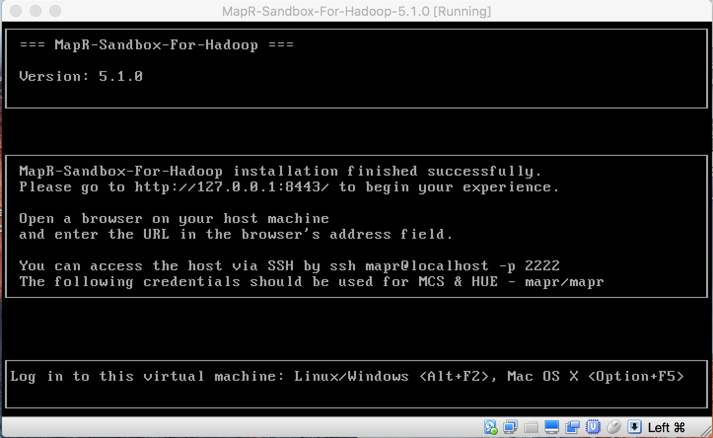
NOTE: you need to press the “command” key in MacOS or the right “control” key in Windows to get your mouse cursor out of the console window.
Once the Sandbox is started, take a look at what comes up. The Sandbox itself is an environment where you can interact with your data, but if you go to http://127.0.0.1:8443/ you can access the file system and familiarize yourself with how the data is stored.
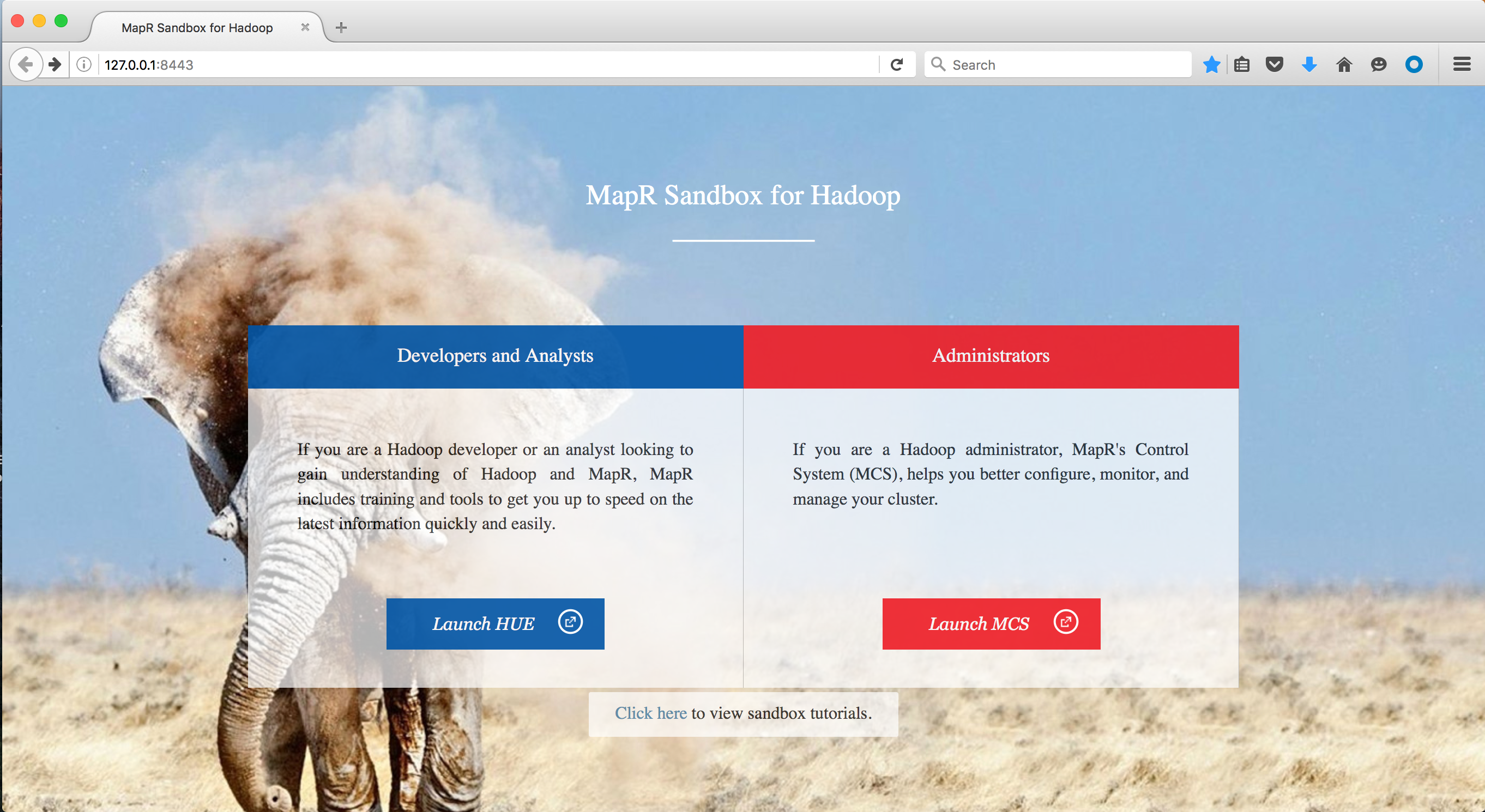
For this tutorial, we will be in HUE. Launch HUE and type in the username/password combination: Username:
Username: mapr
Password: mapr
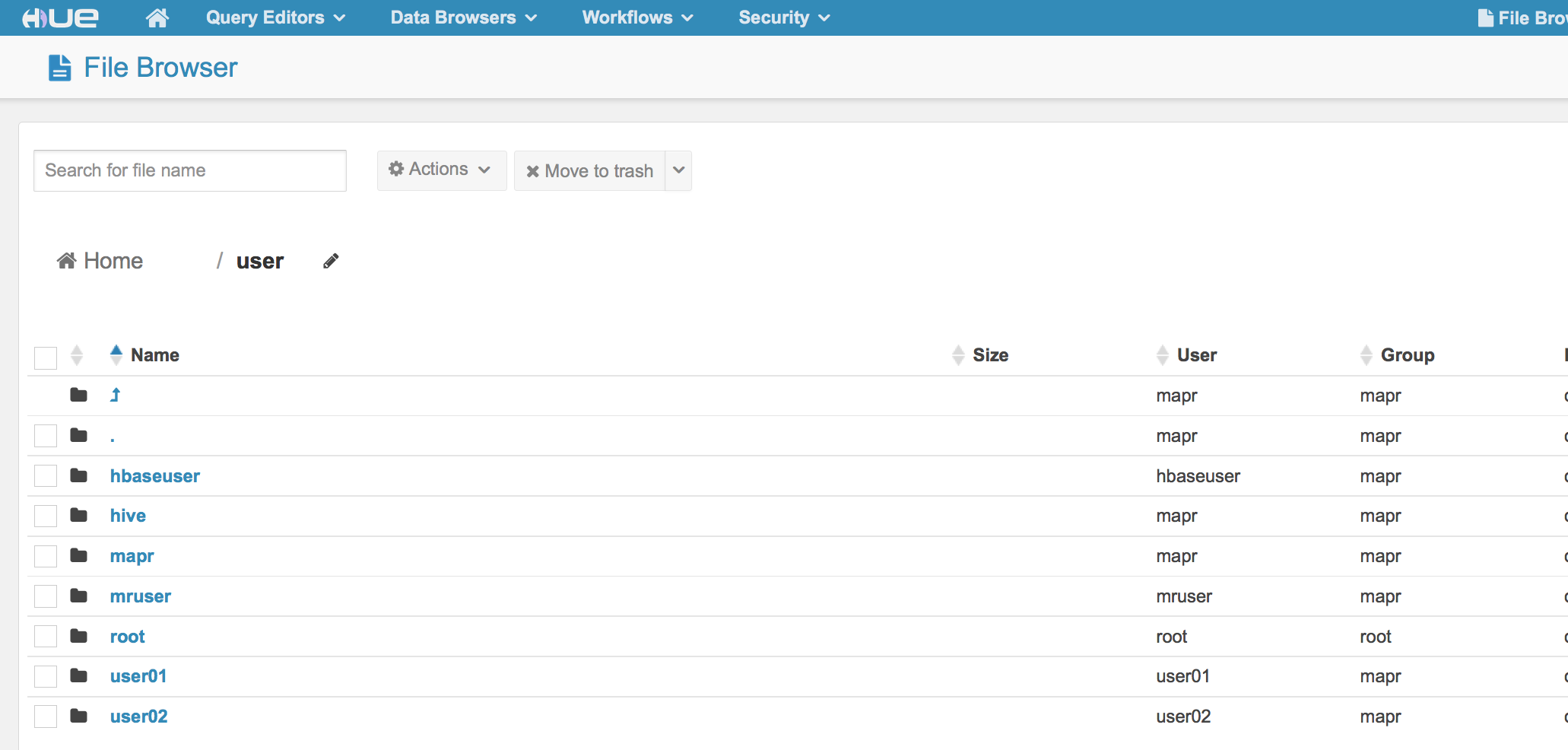
Once HUE opens, go to the file browser:
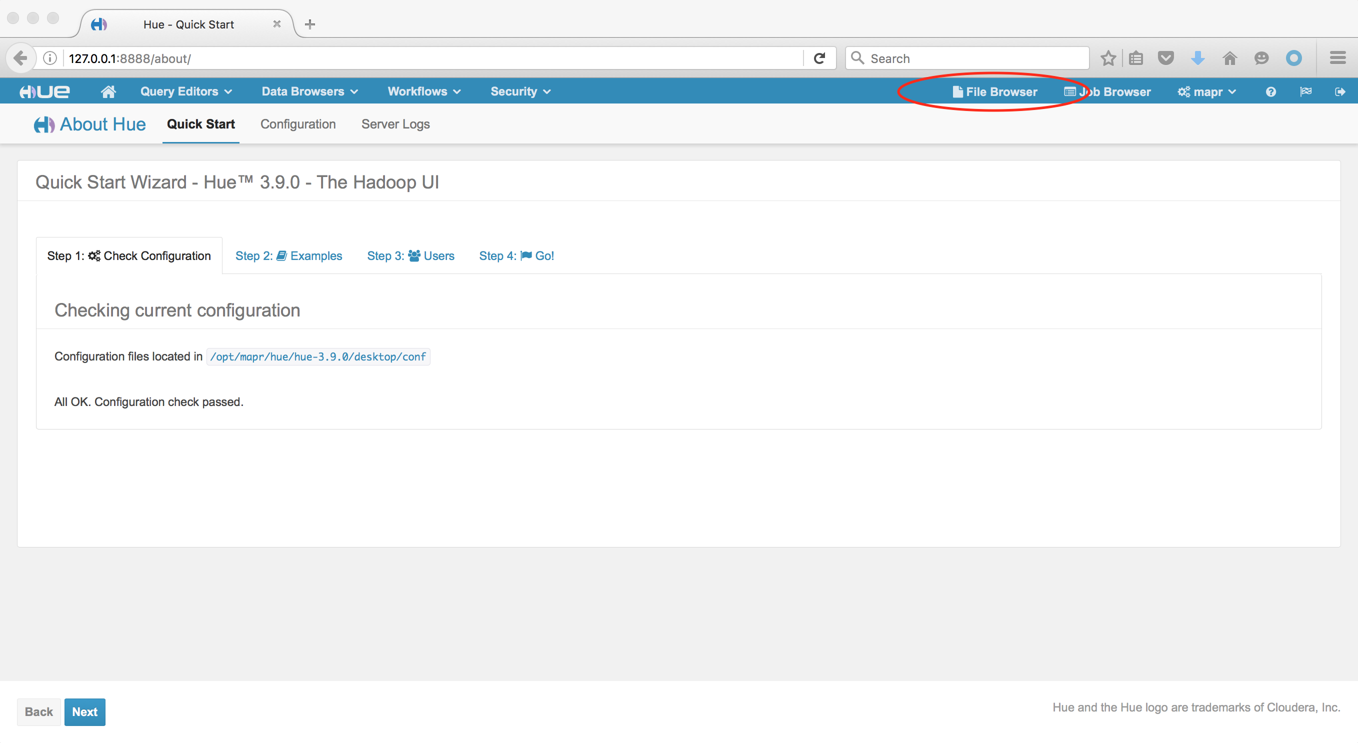
When you are the in the file browser, you will see you are in the /user/mapr directory.
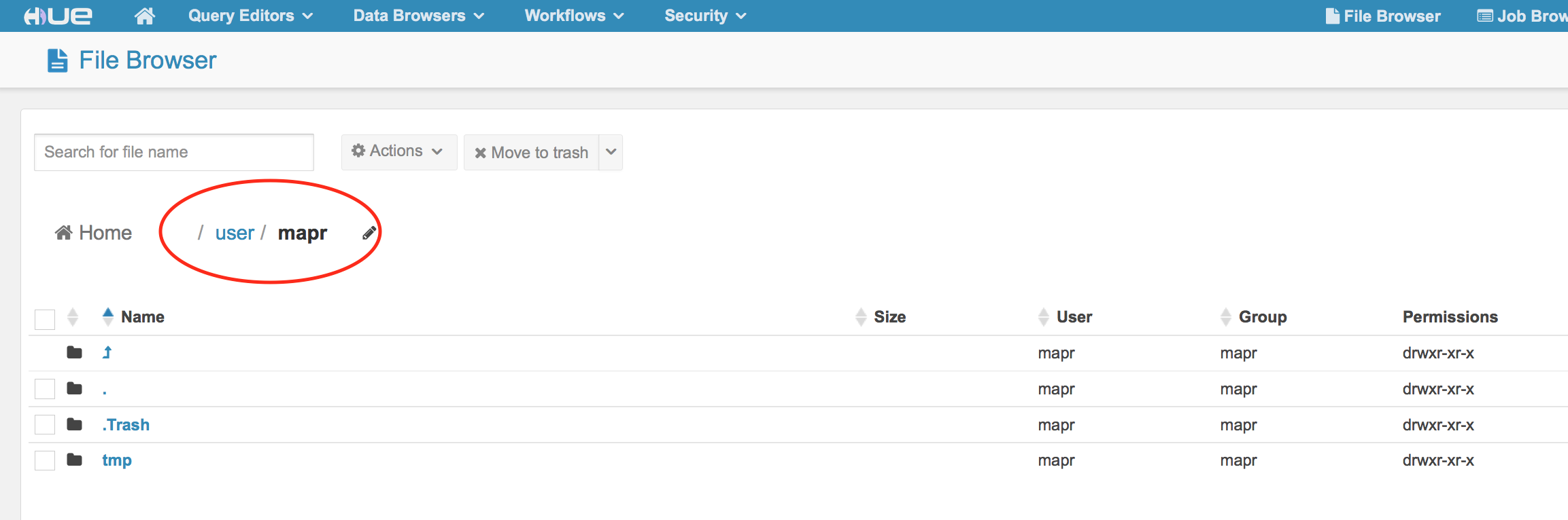
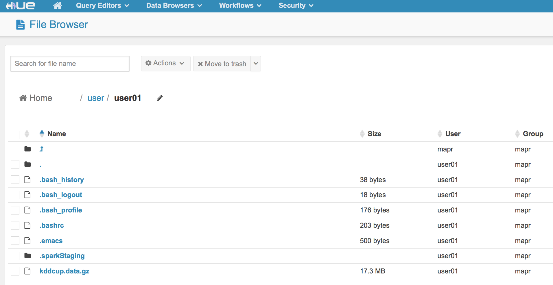
We are going to operate as user01. To get to that directory, click on the /user directory
Make sure you see user01.
Now we have access to user01 within our Sandbox. This is where you can create folders and store data to be used to test out your Spark code. When working with the Sandbox itself, you can use the Sandbox command line if you choose, or you can connect via the terminal or PuTTY on your machine as “user01”. If you choose to connect via a terminal, use ssh and the following command: $ ssh user01@localhost -p 2222 The password is: mapr
Welcome to your Mapr Demo Virtual machine.
[user01@maprdemo ~]$
For this tutorial, I am using a Mac laptop and a terminal application called iTerm2. I could also use my normal default terminal in my Mac as well.
The Sandbox comes with Spark installed. Python is also installed on the Sandbox, and the Python version is 2.6.6.
[user01@maprdemo ~]$ python --version
Python 2.6.6
PySpark uses Python and Spark; however, there are some additional packages needed. To install these additional packages, we need to become the root user for the sandbox. (password is: mapr)
[user01@maprdemo ~]$ su -
Password:
[root@maprdemo ~]#
[root@maprdemo ~]# yum -y install python-pip
[root@maprdemo ~]# pip install nose
[root@maprdemo ~]# pip install numpy
The numpy install might take a minute or two. NumPy and Nose are packages that allow for array manipulation and unit tests within Python.
[root@maprdemo ~]# su - user01
[user01@maprdemo ~]$
PySpark in the Sandbox
To start PySpark, type the following:
[user01@maprdemo ~]$ pyspark --master yarn-client
Below is a screen shot of what your output will approximately look like. You will be in Spark, but with a Python shell¬¬¬.
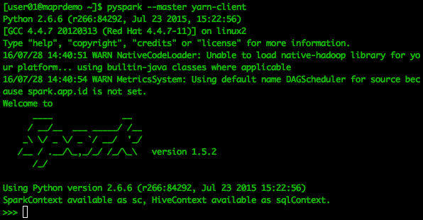
The following code will be executed within PySpark at the >>> prompt.
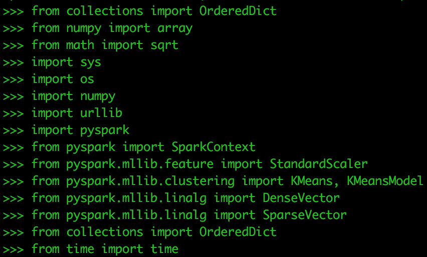
Copy and paste the following to load dependency packages for this exercise:
from collections import OrderedDict
from numpy import array
from math import sqrt
import sys
import os
import numpy
import urllib
import pyspark
from pyspark import SparkContext
from pyspark.mllib.feature import StandardScaler
from pyspark.mllib.clustering import Kmeans, KmeansModel
from pyspark.mllib.linalg import DenseVector
from pyspark.mllib.linalg import SparseVector
from collections import OrderedDict
from time import time
Next,we will check our working directory, put the data into it, and check to make sure it is there.
Check the directory:
os getcwd()

>>>> os.getcwd()
'/user/user01'
Get the Data
f = urllib.urlretrieve ("http://kdd.ics.uci.edu/databases/kddcup99/kddcup.data.gz", "kddcup.data.gz")Check to see the data is in the current working directory
os.listdir('/user/user01')
Now you should see kddcup.data.gz in the directory “user01”. You can also check in HUE.
Data Import and Exploration
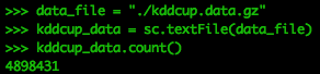
PySpark can import compressed files directly into RDDs.
data_file = "./kddcup.data.gz"
kddcup_data = sc.textFile(data_file)
kddcup_data.count()
Looking at the first 5 records of the RDD
kddcup_data.take(5)

This output is difficult to read. This is because we are asking PySpark to show us data that is in the RDD format. PySpark has a DataFrame functionality. If the Python version is 2.7 or higher, you can utilize the pandas package. However, pandas doesn’t work on Python versions 2.6, so we use the Spark SQL functionality to create DataFrames for exploration.
from pyspark.sql.types import *
from pyspark.sql import DataFrame
from pyspark.sql import SQLContext
from pyspark.sql import Row
kdd = kddcup_data.map(lambda l: l.split(","))
df = sqlContext.createDataFrame(kdd)
df.show(5)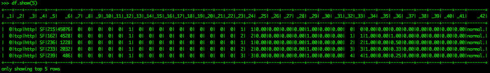
Now we can see the structure of the data a bit better. There are no column headers for the data, as they were not included in the file we downloaded. These are in a separate file and can be appended to the data. That is not necessary for this exercise, as we are more concerned with the groups within the data than the features themselves.
This data has already been labeled, meaning the types of malicious cyber behavior have been assigned to a row. This label is the last feature, _42, in the above screen capture. The first five rows off the dataset are labeled “normal.” However, we should determine the counts of the labels for the entire dataset.
Now let’s get an idea of the different types of labels in this data, and the total number for each label. Let’s time how long this takes.
labels = kddcup_data.map(lambda line: line.strip().split(",")[-1])
start_label_count = time()
label_counts = labels.countByValue()
label_count_time = time()-start_label_count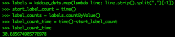
sorted_labels = OrderedDict(sorted(label_counts.items(), key=lambda t: t[1], reverse=True))
for label, count in sorted_labels.items():    #simple for loop
	print label, count
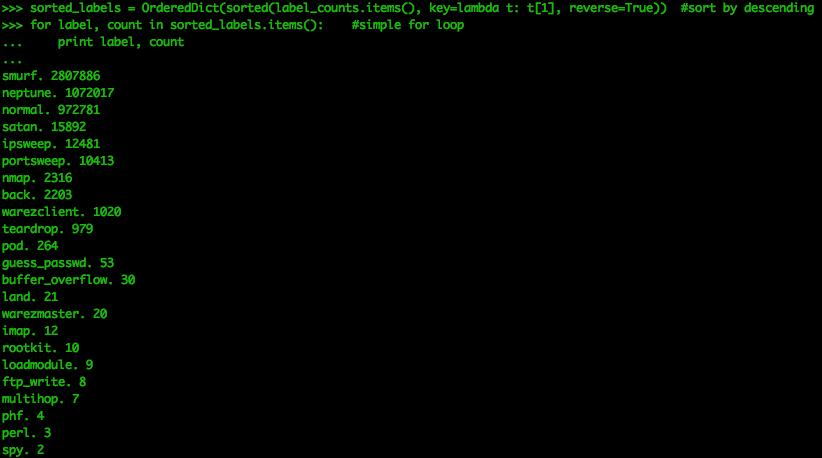
We see there are 23 distinct labels. Smurf attacks are known as directed broadcast attacks, and are a popular form of DoS packet floods. This dataset shows that “normal” events are the third most occurring type of event. While this is fine for learning the material, this dataset shouldn’t be mistaken for a real network log. In a real network dataset, there will be no labels and the normal traffic will be much larger than any anomalous traffic. This results in the data being unbalanced, making it much more challenging to identify the malicious actors.
Now we can start preparing the data for our clustering algorithm.
Data Cleaning
K-means only uses numeric values. This dataset contains three features (not including the attack type feature) that are categorical. For the purposes of this exercise, they will be removed from the dataset. However, performing some feature transformations where these categorical assignments are given their own features and are assigned binary values of 1 or 0 based on whether they are “tcp” or not could be done.
First, we must parse the data by splitting the original RDD, kddcup_data, into columns and removing the three categorical variables starting from index 1 and removing the last column. The remaining columns are then converted into an array of numeric values, and then attached to the last label column to form a numeric array and a string in a tuple.
def parse_interaction(line):
    line_split = line.split(",")
    clean_line_split = [line_split[0]]+line_split[4:-1]
    return (line_split[-1], array([float(x) for x in clean_line_split]))

parsed_data = kddcup_data.map(parse_interaction)
pd_values = parsed_data.values().cache()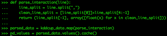
We are putting the values from the parser into cache for easy recall.
The Sandbox does not have enough memory to process the entire dataset for our tutorial, so we will take a sample of the data.
kdd_sample = pd_values.sample(False, .10, 123)
kdd_sample.count()
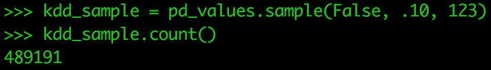
We have taken 10% of the data. The sample() function is taking values without replacement (false), 10% of the total data and is using a the 123 set.seed capability for repeating this sample.
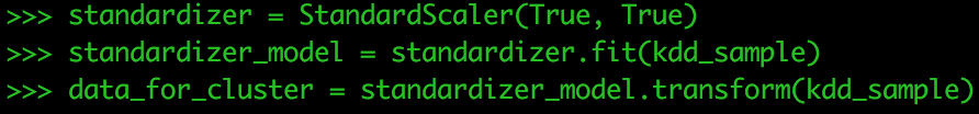
Next, we need to standardize our data. StandardScaler standardizes features by scaling to unit variance and setting the mean to zero using column summary statistics on the samples in the training set. Standardization can improve the convergence rate during the optimization process, and also prevents against features with very large variances exerting an influence during model training.
standardizer = StandardScaler(True, True)
Compute summary statistics by fitting the StandardScaler
standardizer_model = standardizer.fit(kdd_sample)
Normalize each feature to have unit standard deviation.
data_for_cluster = standardizer_model.transform(kdd_sample)
Clustering the data
How is doing k-means in Python’s scikit-learn different from doing it in Spark? Pyspark’s MLlib implementation includes a parallelized variant of the k-means++ method (which is the default for Scikit-Learn’s implementation) called k-means || which is the parallelized version of k-means. In the Scala Data Analysis Cookbook (Packt Publishing 2015), Arun Manivannan gives this explanation of how they differ:
K-means++
Instead of choosing all the centroids randomly, the k-means++ algorithm does the following:
- It chooses the first centroid randomly (uniform)
- It calculates the distance squared of each of the rest of the points from the current centroid
- A probability is attached to each of these points based on how far they are. The farther the centroid candidate is, the higher is its probability.
- We choose the second centroid from the distribution that we have in step 3. On the ith iteration, we have 1+i clusters. Find the new centroid by going over the entire dataset and forming a distribution out of these points based on how far they are from all the precomputed centroids. These steps are repeated over k-1 iterations until k centroids are selected. K-means++ is known for considerably increasing the quality of centroids. However, as we see, in order to select the initial set of centroids, the algorithm goes through the entire dataset k times. Unfortunately, with a large dataset, this becomes a problem.
K-means||
With k-means parallel (K-means||), for each iteration, instead of choosing a single point after calculating the probability distribution of each of the points in the dataset, a lot more points are chosen. In the case of Spark, the number of samples that are chosen per step is 2 * k. Once these initial centroid candidates are selected, a k-means++ is run against these data points (instead of going through the entire dataset).
For this example, we are going to stay with k-means++ because we are still in the sandbox and not a cluster. You will see this in our initialization in the code where it says:
initializationMode="random"
If we wanted to do k-means parallel:
initializationMode="k-means||"
Refer to the MLlib documentation for more info. (http://spark.apache.org/docs/1.6.2/api/python/pyspark.mllib.html#pyspark.mllib.clustering.KMeans)
When performing k-means, the analyst chooses the value of k. However, rather than run the algorithm each time for k, we can package that up in a loop that runs through an array of values for k. For this exercise, we are just doing three values of k. We will also create an empty list called metrics that will store the results from our loop.
k_values = numpy.arange(10,31,10)
metrics = []
One way to evaluate the choice of k is to determine the Within Set Sum of Squared Errors (WSSSE). We are looking for the value of k that minimizes the WSSSE.
def error(point): center = clusters.centers[clusters.predict(point)] denseCenter = DenseVector(numpy.ndarray.tolist(center)) return sqrt(sum([x**2 for x in (DenseVector(point.toArray()) - denseCenter)]))
Run the following in your Sandbox. It could take a while to process, which is why we are only using three values of k.
for k in k_values:
     clusters = Kmeans.train(data_for_cluster, k, maxIterations=4, runs=5, initializationMode="random")
     WSSSE = data_for_cluster.map(lambda point: error(point)).reduce(lambda x, y: x + y)
     results = (k,WSSSE)
     metrics.append(results)

metrics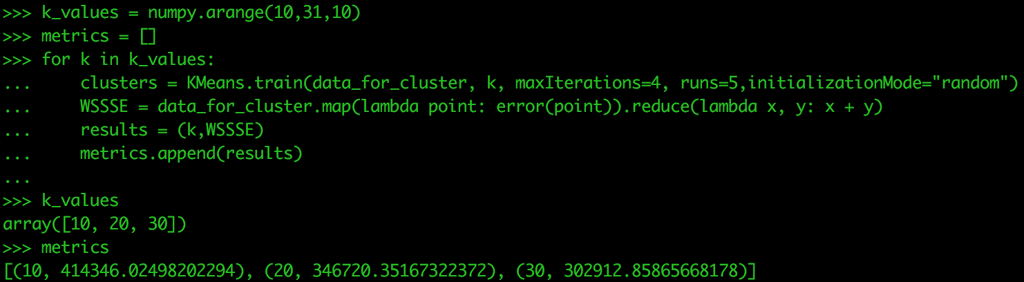
In this case, 30 is the best value for k. Let’s check the cluster assignments for each data point when we have 30 clusters. The next test would be to run for k values of 30, 35, 40. Three values of k is not the most you test on in a single run, but only used for this tutorial.
k30 = Kmeans.train(data_for_cluster, 30, maxIterations=4, runs=5, initializationMode="random")
cluster_membership = data_for_cluster.map(lambda x: k30.predict(x))
cluster_idx = cluster_membership.zipWithIndex()
cluster_idx.take(20)
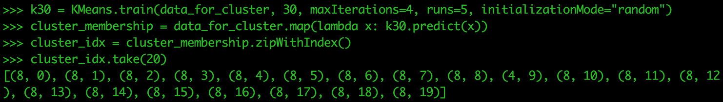
Your results might be slightly different. This is due to the random placement of the centroids when we first begin the clustering algorithm. Performing this many times allows you to see how points in your data change their value of k or stay the same.
I hope you were able to get some hands-on experience using PySpark and the MapR Sandbox. It is an excellent environment to test your code and tune for efficiency. Also, understanding how your algorithm will scale is an important piece of knowledge when transitioning from using PySpark on a local machine to a cluster. The MapR Platform has Spark integrated into it, which makes it easier for developing and then migrating your code into an application. MapR also supports streaming k-means in Spark as opposed to the batch k-means we are performing in this tutorial.
| Reference: | Tutorial: Using PySpark and the MapR Sandbox from our JCG partner Justin Brandenburg at the Mapr blog. |
