During the last part of my career I had a chance to work with Data Scientists having strong skills in Python. My tech background, after a start with C/C++, is in JVM programming languages mostly (but I had to touch several others during my career), so it was a great chance for me to learn more about practical Python, at least in the Machine Learning and Deep Learning spaces. I am no more a full time developer since few years, as I moved to other roles, but this didn’t stop me following my passion for programming languages and staying hands-on with technology in general, not only because I enjoy it, but also because I believe whatever your role is, it is always important to understand the possibilities and the limits of technologies before making any kind of decision.
In this new long series I am going first to share some of the things I have learned about doing time series forecasting through Deep Learning using Python (with Keras and Tensorflow), and finally I will present a follow-up of my book, showing how to do the same with DL4J and/or Keras (with or without Spark). I am going to start today with basic stuff, then I am going to add any time more complexity.
For all of the posts in this series I am going to refer to Python 3. I am going to focus on the time series matters and assuming that you have a working Python 3 environment and know how to install libraries on it.
In this first part, before moving to a DL model implementation, we are going to get familiar with some basic things. The Python libraries involved are pandas, matplotlib and scikit-learn.
What is a time series? It is a sequence of numerical data points indexed in time order. I have dealt (and still deal) with many time series in the last few years (you couldn’t expect otherwise if working in some business such as healthcare, cyber security or manufacturing), so time series analysis and forecasting have been really useful to me. Time series could be univariate (when they present a one-dimension value) or multivariate (when they have multiple observations changing over time). In the first posts of this series I am going to refer to univariate time series only, in order to make the concepts understanding as easier as possible. At a later stage we are going to cover multivariate time series too.
Of course I can’t share production data, so I have picked up a public data set available in Kaggle for these first posts. The data set I am going to use is part of the Advanced Retail Sales Time Series Collection, which is provided and maintained by the Unites States Census Bureau. There are different data sets available as part of the Advance Monthly Retail Trade Survey, which provides indication of sales of retail and food service companies. The one I am using for this post contains the retail sales related to building materials and garden equipment suppliers and dealers.
First thing to do is to load the data set into a pandas DataFrame. The data set contains four features, value, date, realtime_end and realtime_start. The
date feature comes as as string containing dates in the format YYYY-MM-DD. We need to convert those values to dates. We can then define a function for this purpose, to be applied to the date values at loading time:
from pandas import datetime
 def parser(x):
     return datetime.strptime(x, '%Y-%m-%d')
We really need only the first two features (value and date), so when loading from the CSV file, we are going to discard the other two. We need also to specify the column which contains the date values and the parser function to apply:
from pandas import read_csv
 features = ['date', 'value']
 series = read_csv('./advance-retail-sales-building-materials-garden-equipment-and-supplies-dealers.csv', usecols=features, header=0, parse_dates=[1], index_col=1, squeeze=True, date_parser=parser)
When can now have a look at a sample of the rows in the DataFrame:
series.head()
The output should be something like this:
date
1992-01-01 10845
1992-02-01 10904
1992-03-01 10986
1992-04-01 10738
1992-05-01 10777
Name: value, dtype: int64
We can also plot the time series through matplotlib:
series.plot()
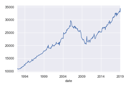
The data set contains the monthly retail data from January 1992 to date. We need to split the data set into train and test data. We are going to use 70% of the data (years from 1992 to 2010) for training and the remaining 30% (years from 2011 to date) for validation:
X = series.values
 train, test = X[0:-98], X[-98:]
One way to evaluate time series forecasting models using a test data set is the so called walk-forward validation. No model training is required because basically we get predictions by moving through the test data set time step by time step. Which, translated in quick and dirty Python code is:
history = [train_value for train_value in train]
 predictions = list()
 for idx in range(len(test)):
     predictions.append(history[-1])
     history.append(test[idx])
At the end of the walk-forward validation, if we plot in a single chart both the observed and the predicted values:
import numpy as np
 x_axis_values = np.arange(1, 99)
 pyplot.figure(figsize=[13,8])
 pyplot.plot(x_axis_values, test, label = 'Observed')
 pyplot.plot(x_axis_values, predictions, label = 'Predicted')
 pyplot.legend()
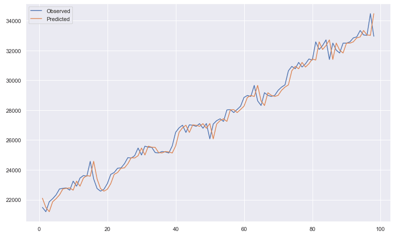
at a glance the situations seems good. But if we do a performance check:
from sklearn.metrics import mean_squared_error
 from math import sqrt
 rmse = sqrt(mean_squared_error(test, predictions))
 print('RMSE: %.3f' % rmse)
we can see that the resulting RMSE (root-mean-square deviation) isn’t so good: RMSE: 518.697
In the next posts of this series you will learn how to build more robust and efficient models through LSTMs.
Published on Java Code Geeks with permission by Guglielmo Iozzia, partner at our JCG program. See the original article here: Time Series & Deep Learning (Part 1 of N): Basic Stuff Opinions expressed by Java Code Geeks contributors are their own. |
