EDITORIAL NOTE: Amazon DynamoDB is a fully managed proprietary NoSQL database services that is offered by Amazon.com as part of the Amazon Web Services portfolio.
DynamoDB exposes a similar data model and derives its name from Dynamo, but has a different underlying implementation. Dynamo had a multi-master design requiring the client to resolve version conflicts and DynamoDB uses synchronous replication across multiple datacenters for high durability and availability.
DynamoDB differs from other Amazon services by allowing developers to purchase a service based on throughput, rather than storage. If Auto Scaling is enabled, then the database will scale automatically. (Source: Wikipedia)
Now, we provide a comprehensive guide so that you can develop your own Amazon DynamoDB based applications. We cover a wide range of topics, from Java Integration and Best Practices, to Backup and Pricing. With this guide, you will be able to get your own projects up and running in minimum time. Enjoy!
1. Introduction
Amazon DynamoDB is a NoSQL database service offered by Amazon as part of its Amazon Web Service (AWS) portfolio. It supports storing, querying, and updating documents and offers SDKs for different programming languages.
DynamoDB supports a key-value data model. Each item (row) in a table is a key-value pair. The primary key is the only required attribute for an item and uniquely identifies each item. Beyond that, DynamoDB is schema-less, i.e. each item can have any number of attributes and the types of the attributes can vary from item to item. One cannot only query the primary key but it is possible to setup secondary indexes (global and local) to query other attributes.
These secondary indexes can be created at any time, meaning that you do not have to define them when you create the table.
As DynamoDB uses the AWS infrastructure, it can scale automatically and therewith handle higher throughput rates and increase the available storage at runtime. The AWS infrastructure also enables high availability and data replication
between different regions in order to serve data more locally.
2. Concepts
2.1 Tables, Items, and Attributes
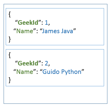
Tables are used to store data and represent a collection of items. The following figure depicts a table with two items. Each item has a primary key (here: GeekId) and an attribute called “Name”.
Items are similar to rows in other database systems, but in DynamoDB, there is no limit to the number of items that can be stored in one table. The attributes are similar to columns in relational databases, but as DynamoDB is schema-less,
it does not restrict the data type of each attribute nor does it force the definition of all possible attributes beforehand. Beyond the example above, attributes can also be nested, i.e. for example, an attribute address can have sub-attributes named
Street or City. Supported are up to 32 levels of nested attributes.
2.2 Primary Keys
The primary key identifies each item within a table uniquely. DynamoDB supports two different kinds of primary keys:
- Partition key / Hash attribute
- Partition key and sort key / Hash and range attribute
The first type is a scalar value, i.e. an attribute that can hold only a single value of the type’s string, number and binary. DynamoDB computes a hash over the attribute’s value in order to determine the partition in which the corresponding item will be stored. A table is divided into different partitions, each partition stores a subset of all values. This way DynamoDB can work concurrently on different partitions and divide larger tasks into smaller ones.
The second type of primary key consists of two values: a partition key and a sort key. It therefore is a kind of compound key. Like in the first case, the partition key is used to determine the partition the current item is stored in. In contrast to a table with only a partition key, the items in a table with an additional sort key are stored in sorted order by the sort key. This way of storing the data provides more flexibility in querying the data as range queries can be performed more efficiently. If you would store for example the projects of an employee in one table and define the project as sort key, DynamoDB can serve queries that should deliver a subset of projects of an employee more easily. In such kind of tables, two items with the same partition key can exist, but they must have different sort keys. The tuple of (partition key / sort key) must be unique for each item.
As the partition of an item is computed by applying a hash function to the partition key, the partition key is often called “hash attribute”. In addition, because the sort key eases range queries, it often called “range attribute”.
2.3 Secondary Indexes
Often it is required to query data not only by its primary key, but additionally also by other attributes. To speed up such kind of queries, indexes can be created that contain a subset of attributes of the base table. These indexes can then be queried much faster.
DynamoDB distinguishes two different kinds of secondary indexes:
- Global secondary index
- Local secondary index
A global secondary index has a partition key and sort key that can be different from the one of the base table. It is called a “global” index because queries on this index can span all the data in the base table.
In contrast to global secondary indexes, a local secondary index has the same partition key as the base table but a different sort key. As base table and index have the same partition key, all partitions of the base table have a corresponding partition in the index. Hence, the partitions of the index are “local” to the base table’s partitions.
When deciding whether an index should be global or local, one must consider a few aspects. While local indexes can only have compound keys that consist of primary key and sort key, a global index can also have a primary key that consists only of a partition key. The partition key of the global index can be different from the one of the local index. Unfortunately the size of all local indexes is limited (currently 10GB), whereas global indexes do not have any size restriction.
Another shortcoming of local indexes is that you can only create them when its base table is created. Creating a local index when the base table has already been created is not supported. This is different to global indexes, which can be created and deleted at any time. On the other hand, local indexes have the advantage that they provide strong consistency, while global indexes only support eventual consistency. Beyond that, local indexes allow us to fetch data from the base table during queries, which is not supported for global indexes.
The number of indexes per table is limited to five for global and local indexes likewise. When deleting a table, all its indexes are also removed.
2.4 Streams
An interesting feature of DynamoDB are streams. DynamoDB creates a new record and inserts it into the stream in case one of the following events happens:
- A new item is added to the table.
- An item in the table is updated.
- An item is removed from the table.
The record contains next to metadata about the event like its timestamp also a copy of the item at the moment of the event. In case of updates, it even contains an image before and after the update. If the stream is enabled on table, it can be used to implement triggers. This way you can perform an action in case one of the events above happens. One can imagine to send for example an email if a new order is stored in a table or to order new articles in case it gets out of stock. This feature can also be used to implement data replication or what is known in other database system as materialized views.
Records in a stream are removed automatically after 24 hours.
3. Java SDK
3.1 Setup
In this tutorial we are going to use maven as build system. Hence, the first step is to create a local maven project. This can be done by invoking the following command on the command line:
mvn archetype:generate -DgroupId=com.javacodegeeks.aws -DartifactId=dynamodb -DarchetypeArtifactId=maven-archetype-quickstart -DinteractiveMode=false
This creates a simple maven project with the following layout in the file system:
|-- pom.xml
`-- src
    |-- main
    |   `-- java
    |       `-- com
    |           `-- javacodegeeks
    |               `-- aws
    |                   `-- App.java
    `-- test
        `-- java
            `-- com
                `-- javacodegeeks
                    `-- aws
                        `-- AppTest.java
First, we edit the pom.xml file and add the following dependency:
<dependency>
	<groupId>com.amazonaws</groupId>
	<artifactId>DynamoDBLocal</artifactId>
	<version>[1.11,2.0)</version>
</dependency>
This tells maven to download a local version of DynamoDB (and all of its dependencies) into our local maven repository such that we can create a local running instance of the database. This local database has the advantage that we can issue as many requests as we want without having to pay for it. Once our application has been developed and tested, we can modify it to use a DynamoDB instance running in the AWS infrastructure.
As the dependency above is not available in the Central Maven Repository, we have to add Amazon’s repository to the pom.xml file:
<repositories>
	<repository>
		<id>dynamodb-local-oregon</id>
		<name>DynamoDB Local Release Repository</name>
		<url>https://s3.eu-central-1.amazonaws.com/dynamodb-local-frankfurt/release</url>
	</repository>
</repositories>
The example above uses the repository located in Frankfurt, Germany. If you prefer a different location that is closer to you, you can chose one from the list here. This page also explains how to download a distribution of DynamoDB that can be started locally from command line, if you prefer this. In this tutorial, we are using the maven dependency, because it allows us to start an in-memory instance directly from our code.
As the local database instance uses native libraries, it needs them extracted in a local directory. We utilize maven’s dependency plugin to extract the necessary dependencies into the target directory of the build:
<build>
	<plugins>
		<plugin>
			<groupId>org.apache.maven.plugins</groupId>
			<artifactId>maven-dependency-plugin</artifactId>
			<version>3.0.1</version>
			<executions>
				<execution>
					<id>copy-dependencies</id>
					<phase>process-test-resources</phase>
					<goals>
						<goal>copy-dependencies</goal>
					</goals>
					<configuration>
						<outputDirectory>${project.build.directory}/dependencies</outputDirectory>
						<overWriteReleases>false</overWriteReleases>
						<overWriteSnapshots>false</overWriteSnapshots>
						<overWriteIfNewer>true</overWriteIfNewer>
					</configuration>
				</execution>
			</executions>
		</plugin>
	</plugins>
</build>
To start our sample application within the maven build, the following profile uses the maven exec plugin to start a task:
    <profiles>
        <profile>
            <id>exec</id>
            <build>
                <plugins>
                    <plugin>
                        <groupId>org.codehaus.mojo</groupId>
                        <artifactId>exec-maven-plugin</artifactId>
                        <version>1.6.0</version>
                        <executions>
                            <execution>
                                <phase>package</phase>
                                <configuration>
                                    <executable>java</executable>
                                    <arguments>
                                        <argument>-cp</argument>
                                        <classpath/>
                                        <argument>-Dsqlite4java.library.path=${basedir}/target/dependencies</argument>
                                        <argument>com.javacodegeeks.aws.App</argument>
                                        <argument>${app.task}</argument>
                                    </arguments>
                                </configuration>
                                <goals>
                                    <goal>exec</goal>
                                </goals>
                            </execution>
                        </executions>
                    </plugin>
                </plugins>
            </build>
        </profile>
    </profiles>
The application we will develop uses as first argument the name of a “task”. In our snippet above, we define this task by using a maven property. This property can be set on the command line together with the activation of the profile:
mvn package -Pexec -Dapp.task=ListTables
To start a local server from Java code encompasses a few lines of code:
DynamoDBProxyServer server = ServerRunner
	.createServerFromCommandLineArgs(new String[]{
		"-dbPath", System.getProperty("user.dir") + File.separator + "target",
		"-port", port
		});
server.start();
The class ServerRunner has the static method createServerFromCommandLineArgs() that takes a number of arguments. In our example we define that the server should use the specified directory to store its files and listen on the specified port.
Once the server is started, we can connect using the AmazonDynamoDBClientBuilder:
AmazonDynamoDB dynamodb = AmazonDynamoDBClientBuilder
	.standard()
	.withEndpointConfiguration(
		new AwsClientBuilder.EndpointConfiguration("http://localhost:" + port, "us-west-2")
	)
	.withCredentials(new AWSStaticCredentialsProvider(new AWSCredentials() {
		@Override
		public String getAWSAccessKeyId() {
			return "dummy";
		}

		@Override
		public String getAWSSecretKey() {
			return "dummy";
		}
	}))
	.build();
The builder method standard() constructs a database instance with default configuration values. An endpoint is configured using an instance of AwsClientBuilder.EndpointConfiguration and passing the URL and the Amazon region as arguments. As we have started the server on localhost, we configured the endpoint on the same host. In real world applications, you would use the IP address or name of the host running the DynamoDB instance.
The local database ignores the Amazon region, hence we can provide the static string us-west-2. The same is true for access key and secret key. Dummy values as shown above are sufficient to connect. Anyhow, in real world scenarios you would not provide them hard coded but use a different provider. The SDK ships with providers that read the values from environment variables, system properties, profile files etc. One is free to implement a specific provider if necessary. More details on this topic can be found here.
Finally a call of build() creates a new instance of AmazonDynamoDB, the client object we will use to interact with the database.
Now that we know how to start a local database and how to connect, we can surround the code snippets above by statements that start the code of a Java class by looking up its name per reflection and pass the constructed instance of AmazonDynamoDB to it:
public static void main(String[] args) throws Exception {
	if (args.length < 1) {
		System.err.println("Please provide the task to run.");
		System.exit(-1);
	}
	String taskName = args[0];
	try {
		Class<?> aClass = Class.forName("com.javacodegeeks.aws.tasks." + taskName);
		Object newInstance = aClass.newInstance();
		if (newInstance instanceof Task) {
			Task task = (Task) newInstance;
			String[] argsCopy = new String[args.length - 1];
			System.arraycopy(args, 1, argsCopy, 0, args.length - 1);

			AmazonDynamoDB dynamodb = null;
			String port = "8000";
			DynamoDBProxyServer server = null;
			try {
				server = ServerRunner.createServerFromCommandLineArgs(new String[]{ "-inMemory", "-port", port});
				server.start();
				dynamodb = AmazonDynamoDBClientBuilder.standard()
						.withEndpointConfiguration(new AwsClientBuilder.EndpointConfiguration("http://localhost:" + port, "us-west-2"))
						.withCredentials(new AWSStaticCredentialsProvider(new AWSCredentials() {
							@Override
							public String getAWSAccessKeyId() {
								return "dummy";
							}

							@Override
							public String getAWSSecretKey() {
								return "dummy";
							}
						}))
						.build();
				task.run(argsCopy, dynamodb);
			} finally {
				if(server != null) {
					server.stop();
				}
				if(dynamodb != null) {
					dynamodb.shutdown();
				}
			}
		} else {
			System.err.println("Class " + aClass.getName() + " does not implement interface " + Task.class.getName() + ".");
		}
	} catch (ClassNotFoundException e) {
		System.err.println("No task with name '" + taskName + " available.");
	} catch (InstantiationException | IllegalAccessException e) {
		System.err.println("Cannot create instance of task '" + taskName + ": " + e.getLocalizedMessage());
	}
}
This allows us to easily add more tasks to the application without writing the same code repeatedly. We also pass additional arguments provided on the command line to the task, such that we can provide further information to it.
If you do not want to hard code the host name and the port, you can easily adjust the sample code above to your needs.
3.2 Tables
In this section, we are going to see how to work with tables. The simplest operation is to list all available tables. This can be done using the following “task”:
public class ListTables implements Task {
    @Override
    public void run(String[] args, AmazonDynamoDB dynamodb) {
        ListTablesResult listTablesResult = dynamodb.listTables();
        List<String> tableNames = listTablesResult.getTableNames();
        System.out.println("Number of tables: " + tableNames.size());
        for (String tableName : tableNames) {
            System.out.println("Table: " + tableName);
        }
    }
}
As we can see the AmazonDynamoDB has a method called listTables() that returns a ListTablesResult object. This object reveals the list of tables by invoking its method getTableNames(). By putting this class into the package com.javacodegeeks.aws.tasks we can invoke it as part of the maven build:
mvn package -Pexec -Dapp.task=ListTables
This will output something like:
[INFO] --- exec-maven-plugin:1.6.0:exec (default) @ dynamodb ---
Initializing DynamoDB Local with the following configuration:
Port:   8000
InMemory:       true
DbPath: null
SharedDb:       false
shouldDelayTransientStatuses:   false
CorsParams:     *

Number of tables: 0
As expected, our instance does not have any tables yet. However, we can create a first table using the following code:
public class CreateProductTable implements Task {

    @Override
    public void run(String[] args, AmazonDynamoDB dynamodb) {

        ArrayList<AttributeDefinition> attributeDefinitions = new ArrayList<>();
        attributeDefinitions.add(new AttributeDefinition()
                .withAttributeName("ID").withAttributeType("S"));

        ArrayList<KeySchemaElement> keySchema = new ArrayList<>();
        keySchema.add(new KeySchemaElement()
                .withAttributeName("ID").withKeyType(KeyType.HASH));

        CreateTableRequest createTableReq = new CreateTableRequest()
                .withTableName("Product")
                .withAttributeDefinitions(attributeDefinitions)
                .withKeySchema(keySchema)
                .withProvisionedThroughput(new ProvisionedThroughput()
                        .withReadCapacityUnits(10L)
                        .withWriteCapacityUnits(5L));
        CreateTableResult result = dynamodb.createTable(createTableReq);
        System.out.println(result.toString());
    }
}
First, we define the attributes of the table, but we only define attributes that are part of the key. In this simple case, we will create a table to manage the products of our company; hence, we will name the table “Product” and use an artificial primary key called ID. This key is of type string, which is why we chose S as attribute type. The list of KeySchemaElement is filled with one item that defines the ID attribute as hash key.
When creating a new table one must always specify the initial read and write capacity. It is possible to let Amazon auto-scale the instance when running in the AWS cloud, but even in this case you must specify these two rates when creating the table. It is also possible to adjust these settings later when you applications scales. Read capacity means the number of strongly consistent reads per second or two eventually consistent reads per second. In our example code above we specify that we need 10 strongly consistent reads per second (or 20 eventually consistent reads).
The difference between these types of reads is that strongly consistent reads ensure that the latest written data is returned, while eventual consistency means that a read may return stale data. Repeating the same eventual consistent read a few seconds later may return values that are more current. As AWS distributes the partitions of a table over the AWS cloud, using strong consistent reads requires that all prior write operations are included in the result. Such kind of read does not return a valid result in case of network delays or outages.
On the other hand the write capacity defines the number of 1KB writes per second. Packages of data that are smaller than 1KB are rounded up, hence writing only 500 bytes is counted as a 1KB write. Our example code above tells DynamoDB to scale the system such that we can write up to 5 times per second about 1KB of data.
The return value of an invocation of createTable() contains a description of the table:
{
	TableDescription: {
		AttributeDefinitions: [{
			AttributeName: ID,
			AttributeType: S
		}],
		TableName: Product,
		KeySchema: [{
			AttributeName: ID,
			KeyType: HASH
		}],
		TableStatus: ACTIVE,
		CreationDateTime: Sun Sep 10 13:41:10 CEST 2017,
		ProvisionedThroughput: {
			LastIncreaseDateTime: ThuJan0101: 00: 00CET1970,
			LastDecreaseDateTime: ThuJan0101: 00: 00CET1970,
			NumberOfDecreasesToday: 0,
			ReadCapacityUnits: 10,
			WriteCapacityUnits: 5
		},
		TableSizeBytes: 0,
		ItemCount: 0,
		TableArn: arn: aws: dynamodb: ddblocal: 000000000000: table/Product,

	}
}
The output reflects the changes we have made: The attribute ID is defined as string and hash key, the table is already active and we can see the defined read and write rates. We also get information about the number of items stored in the table and the table’s size.
3.3 Items
Now that we a table, we can insert some sample data. The following “task” inserts two products into the table Product:
public class InsertProducts implements Task {
    @Override
    public void run(String[] args, AmazonDynamoDB dynamodb) {
        DynamoDB dynamoDB = new DynamoDB(dynamodb);
        Table table = dynamoDB.getTable("Product");

        String uuid1 = UUID.randomUUID().toString();
        Item item = new Item()
                .withPrimaryKey("ID", uuid1)
                .withString("Name", "Apple iPhone 7")
                .withNumber("Price", 664.9);
        table.putItem(item);

        String uuid2 = UUID.randomUUID().toString();
        item = new Item()
                .withPrimaryKey("ID", uuid2)
                .withString("Name", "Samsung Galaxy S8")
                .withNumber("Price", 543.0);
        table.putItem(item);

        item = table.getItem("ID", uuid1);
        System.out.println("Retrieved item with UUID " + uuid1 + ": name="
                + item.getString("Name") + "; price=" + item.getString("Price"));
        item = table.getItem("ID", uuid2);
        System.out.println("Retrieved item with UUID " + uuid2 + ": name="
                + item.getString("Name") + "; price=" + item.getString("Price"));

        table.deleteItem(new PrimaryKey("ID", uuid1));
        table.deleteItem(new PrimaryKey("ID", uuid2));

        System.out.println(table.describe());
    }
}
First, we create an instance of DynamoDB. This class is the entry point into the “Document API” and provides methods for listing tables writing items. Here we utilize its method getTable() to retrieve a reference to the DynamoDB table. This table object has the method putItem() to store an item under the specified primary key. In this simple example, we are going to use an UUID as product ID and provide it to the item’s withPrimaryKey() method. Helper methods like withString() or withNumber() allows us to provide additional attributes. Please note that these attributes do not need to be specified when creating the table. This allows handling the table schema-less.
After having put two items into the table, we retrieve them back by querying the database for the specific primary key. We also output the two additional attributes we have inserted before. This will produce an output similar to the following:
Retrieved item with UUID 7dc5be93-213b-4b16-95f9-5ee7381b219d: name=Apple iPhone 7; price=664.9
Retrieved item with UUID 06fbf030-93f0-48ca-805f-2e627d72faf4: name=Samsung Galaxy S8; price=543
Finally we remove the two items by using the method deleteItem() and pass the primary key to be deleted. To be sure that everything works as expected, we can verify the output of the describe() method:
{
	TableDescription: {
		AttributeDefinitions: [{
			AttributeName: ID,
			AttributeType: S
		}],
		TableName: Product,
		KeySchema: [{
			AttributeName: ID,
			KeyType: HASH
		}],
		TableStatus: ACTIVE,
		CreationDateTime: Sun Sep 10 13:41:10 CEST 2017,
		ProvisionedThroughput: {
			LastIncreaseDateTime: Thu Jan 01 01:00:00 CET 1970,
			LastDecreaseDateTime: Thu Jan 01 01:00:00 CET 1970,
			NumberOfDecreasesToday: 0,
			ReadCapacityUnits: 10,
			WriteCapacityUnits: 5
		},
		TableSizeBytes: 0,
		ItemCount: 0,
		TableArn: arn: aws: dynamodb: ddblocal: 000000000000: table/Product,

	}
}
We already anticipated that the table has a size of zero bytes and that no items are stored in it. Beyond that, we do not find anything about the two additional attributes we have inserted before. But this is clear, because in a schema-less database like DynamoDB the table structure does not know about all available attributes at runtime. It only manages the essential data about the primary key used to identify each item uniquely.
Up to now, we have seen how to create, read and delete data. To implement a fully functional application, we still need to update data. The following code shows how to do that:
UpdateItemSpec updateSpec = new UpdateItemSpec()
		.withPrimaryKey(new PrimaryKey("ID", uuid1))
		.withUpdateExpression("set Price = :priceNew")
		.withConditionExpression("Price = :priceOld")
		.withValueMap(new ValueMap()
						.withNumber(":priceOld", 664.9)
						.withNumber(":priceNew", 645.9)
		);
table.updateItem(updateSpec);

item = table.getItem("ID", uuid1);
System.out.println("Retrieved item with UUID " + uuid1 + ": name="
		+ item.getString("Name") + "; price=" + item.getString("Price"));
If put into the class InsertProducts above directly after retrieving the items, it will update the first item’s price in case it has a certain value. Therefore we define the expression set Price = :priceNew as update expression and the expression Price = :priceOld as condition. The values for the variables :priceNew and :priceOld are defined using a ValueMap. Passing the UpdateItemSpec to an invocation of updateItem() lets DynamoDB update the item’s price to 645.9 if its current price is 664.9. The following item retrieval outputs this on the console to verify that everything worked as expected.
3.4 Batch operations
Often, especially when existing systems are migrated, large amounts of requests have to be processed in a short time frame. Instead of issuing all these requests as single ones, the batch operations allow to collect a certain amount of operations and send them with one request to the database. This reduces the overhead of sending the request and waiting for a response. For large sets of operations, this can improve application performance significantly.
The following code demonstrates how to batch insert the two products we have inserted before one after the other:
public class BatchInsertProducts implements Task {
    @Override
    public void run(String[] args, AmazonDynamoDB dynamodb) {
        DynamoDB dynamoDB = new DynamoDB(dynamodb);

        String uuid1 = UUID.randomUUID().toString();
        String uuid2 = UUID.randomUUID().toString();
        TableWriteItems tableWriteItems = new TableWriteItems("Product")
                .withItemsToPut(new Item()
                                .withPrimaryKey("ID", uuid1)
                                .withString("Name", "Apple iPhone 7")
                                .withNumber("Price", 664.9),
                        new Item()
                                .withPrimaryKey("ID", uuid2)
                                .withString("Name", "Samsung Galaxy S8")
                                .withNumber("Price", 543.0));

        BatchWriteItemSpec spec = new BatchWriteItemSpec()
                .withProgressListener(new ProgressListener() {
                    @Override
                    public void progressChanged(ProgressEvent progressEvent) {
                        System.out.println(progressEvent.toString());
                    }
                })
                .withTableWriteItems(tableWriteItems);
        BatchWriteItemOutcome outcome = dynamoDB.batchWriteItem(spec);
        System.out.println("Unprocessed items: " + outcome.getUnprocessedItems().size());

        TableKeysAndAttributes tableKeyAndAttributes = new TableKeysAndAttributes("Product")
                .withPrimaryKeys(
                        new PrimaryKey("ID", uuid1),
                        new PrimaryKey("ID", uuid2));
        BatchGetItemSpec getSpec = new BatchGetItemSpec()
                .withProgressListener(new ProgressListener() {
                    @Override
                    public void progressChanged(ProgressEvent progressEvent) {
                        System.out.println(progressEvent.toString());
                    }
                })
                .withTableKeyAndAttributes(tableKeyAndAttributes);
        BatchGetItemOutcome batchGetItemOutcome = dynamoDB.batchGetItem(getSpec);
        System.out.println("Unprocessed keys: " + batchGetItemOutcome.getUnprocessedKeys().size());

        BatchGetItemResult batchGetItemResult = batchGetItemOutcome.getBatchGetItemResult();
        Map<String, List<Map<String, AttributeValue>>> responses = batchGetItemResult.getResponses();
        for (Map.Entry<String, List<Map<String, AttributeValue>>> entry : responses.entrySet()) {
            String tableName = entry.getKey();
            System.out.println("Table: " + tableName);
            List<Map<String, AttributeValue>> items = entry.getValue();
            for (Map<String, AttributeValue> item : items) {
                for (Map.Entry<String, AttributeValue> itemEntry : item.entrySet()) {
                    System.out.println("\t " + itemEntry.getKey() + "=" + itemEntry.getValue());
                }
            }
        }

        Table table = dynamoDB.getTable("Product");
        table.deleteItem(new PrimaryKey("ID", uuid1));
        table.deleteItem(new PrimaryKey("ID", uuid2));
    }
}
Again, we are using the “Document API” of the SDK by creating an instance of DynamoDB. This allows us to call its method batchWriteItem() with an instance of BatchWriteItemSpec as argument. This specification of a batch request takes of course a list of items (here represented as TableWriteItems), but additionally also a progress listener. This way our application gets informed about updates of the batch process. This is helpful when loading huge amounts of data into the database.
The instance of TableWriteItems gets the name of the table as argument to the constructor and the list of Items as parameters to its method withItemsToPut(). Two small items are of course not representative for a batch process, but it should be sufficient for demonstrating how the API works. Please note that you must comply to the write capacity defined when the table was created. Hence, it may happen that the batch process triggers a throttling process on the AWS side, when writing to fast into the database. In our case, this will not happen, because we have requested up to 10 write operations per second, but when working with big data sets you may experience this. In this case, you must check for the number of unprocessed items. It is returned as return value of the method batchWriteItem(). In case there are unprocessed items, one must try a second time to insert them.
The batch API also allows retrieving large sets of items. Again, we have to check that we do not violate the specified read capacity of the table. However, in our small example this should not happen. Retrieving large sets of items can be done by invoking the method batchGetItem() with an instance of BatchGetItemSpec. Like for the write case, we can pass a ProgressListener. Additionally we must also pass the list of items to retrieve. In this case we provide them in form of a list of PrimaryKey objects. The name of the table can be passed to the constructor of TableKeysAndAttributes. This way one can even specify lists of items for different tables.
As a result of an invocation of batchGetItem(), the API returns an instance of BatchGetItemOutcome. The number of unprocessed keys is an indicator if we must retry some of the operations. The outcome also contains the list of items we have requested. The form of this list is a little bit ugly, as it consists of a Map of key/value pairs inside a list. In addition, we have a list for each table, i.e. the list sits again inside a map. Therefore, we must iterate over the map with table names to get first a list of items for each table. This list is again a map for each item with the key/value pairs.
Finally, we delete the two items we have created using the batch API.
3.5 DB Mapper
The last example has shown how tedious the work with maps and lists of attributes can be. To ease the work Amazon also ships a mapping framework that allows mapping normal Java classes to tables in DynamoDB.
Like in other mapping frameworks, Plain Old Java Objects (POJO) are used to transfer the data to the database. Annotations tell the mapping framework how to store the data. The following class shows such a simple annotated POJO:
@DynamoDBTable(tableName="Product")
public class Product {

    private String id;
    private String name;
    private double price;

    @DynamoDBHashKey(attributeName = "ID")
    @DynamoDBAutoGeneratedKey
    public String getId() {
        return id;
    }

    public void setId(String id) {
        this.id = id;
    }

    @DynamoDBAttribute(attributeName="Name")
    public String getName() {
        return name;
    }

    public void setName(String name) {
        this.name = name;
    }

    @DynamoDBAttribute(attributeName="Price")
    public double getPrice() {
        return price;
    }

    public void setPrice(double price) {
        this.price = price;
    }
}
The annotation @DynamoDBTable is used at class level and tells the framework that instances of this class are stored in the table Product. Product follows the bean conventions that all its attributes are accessible through getter and setter methods. Annotations on the getter methods reveal which attributes a product consists of. The annotation @DynamoDBHashKey specifies that the attribute id should hold the hash key of the object. As we have used a different name with regard to lower and uppercase for the id, we have to specify this using the annotation’s attribute attributeName. This way the mapper knows to store the hash key as attribute ID. In the previous examples we have used a random UUID as hash key. Instead of writing the code to create the UUID on our own, we can let the mapper create the random UUID. This is achieved by annotating the getter method of the hash key with @DynamoDBAutoGeneratedKey.
The annotation @DynamoDBAttribute is put at the remaining getter methods of the Product and tells the mapper that a product has a name attribute and a price attribute.
Having implemented this simple POJO class, we can use it to save the same products as in the example with the Item class:
public class MapperInsertProducts implements Task {
    @Override
    public void run(String[] args, AmazonDynamoDB dynamodb) {
        DynamoDBMapper mapper = new DynamoDBMapper(dynamodb);

        Product product1 = new Product();
        product1.setName("Apple iPhone 7");
        product1.setPrice(664.9);
        mapper.save(product1);
        System.out.println("Saved product with ID " + product1.getId());

        Product product2 = new Product();
        product2.setName("Samsung Galaxy S8");
        product2.setPrice(543.0);
        mapper.save(product2);
        System.out.println("Saved product with ID " + product2.getId());

        Product product = mapper.load(Product.class, product1.getId());
        System.out.println("Loaded product: id=" + product.getId() +
                "; name=" + product.getName() +
                "; price=" + product.getPrice());
        product = mapper.load(Product.class, product2.getId());
        System.out.println("Loaded product: id=" + product.getId() +
                "; name=" + product.getName() +
                "; price=" + product.getPrice());

        mapper.delete(product1);
        mapper.delete(product2);
    }
}
In a first step we create an instance of DynamoDBMapper. This class provides all the methods we need to interact with the mapping framework. The second step is to create a Product instance and populate its fields with sample data.
Storing these attributes in the database is done by simply invoking the method save() of the mapper. It also updates the hash key of the item, as we have told the mapping framework to automatically generate it.
To validate that the data has actually been inserted into the database, we call the mapper’s method load(). The first argument tells it which base type we want to be populated with the values from the database. Beyond that the mapper also needs to know the id of the item to load. With this information it can load the data by id and fill a new instance of the Product class with values. Outputting these values to the console lets us verify that we have actually retrieved the same values as we have stored before.
Finally we utilize the mapper’s method delete() to remove the two new products from the table.
3.6 Queries
Because a database is not only used to store but also to query data, we must cover at this point how to issue queries against DynamoDB. Therefore, we need a table with some sample data we can query. This table is created in the first step:
private void createTodoListTable(AmazonDynamoDB dynamodb) {
	ListTablesResult listTablesResult = dynamodb.listTables();
	List<String> tableNames = listTablesResult.getTableNames();
	for (String tableName : tableNames) {
		if ("TodoList".equals(tableName)) {
			DeleteTableRequest deleteTableReq = new DeleteTableRequest().withTableName(tableName);
			dynamodb.deleteTable(deleteTableReq);
			System.out.println("Deleted table " + tableName);
		}
	}

	ArrayList<AttributeDefinition> attributeDefinitions = new ArrayList<>();
	attributeDefinitions.add(new AttributeDefinition()
			.withAttributeName("Category").withAttributeType("S"));
	attributeDefinitions.add(new AttributeDefinition()
			.withAttributeName("CreationDate").withAttributeType("S"));

	ArrayList<KeySchemaElement> keySchema = new ArrayList<>();
	keySchema.add(new KeySchemaElement()
			.withAttributeName("Category").withKeyType(KeyType.HASH));
	keySchema.add(new KeySchemaElement()
			.withAttributeName("CreationDate").withKeyType(KeyType.RANGE));

	CreateTableRequest createTableReq = new CreateTableRequest()
			.withTableName("TodoList")
			.withAttributeDefinitions(attributeDefinitions)
			.withKeySchema(keySchema)
			.withProvisionedThroughput(new ProvisionedThroughput()
					.withReadCapacityUnits(10L)
					.withWriteCapacityUnits(5L));
	CreateTableResult result = dynamodb.createTable(createTableReq);
	System.out.println("Created table " + result.toString());
}

If the table already exists, we remove it. Then we define two attributes of type string (“S”): Category and CreationDate. Date values are stored in DynamoDB as ISO-8601 strings. The category acts as hash key and the creation date as range key.
A simple POJO class maps the class fields to the attributes of the database:
@DynamoDBTable(tableName="TodoList")
public class TodoItem {

    private String category;
    private Date creationDate;
    private String description;
    private String status;

    public static class TodoItemBuilder {

       [...]
    }

    @DynamoDBHashKey(attributeName = "Category")
    public String getCategory() {

        return category;
    }

    public void setCategory(String category) {
        this.category = category;
    }

    @DynamoDBRangeKey(attributeName = "CreationDate")
    public Date getCreationDate() {
        return creationDate;
    }

    public void setCreationDate(Date creationDate) {
        this.creationDate = creationDate;
    }

    @DynamoDBAttribute(attributeName = "Description")
    public void setDescription(String description) {
        this.description = description;
    }

    public String getDescription() {
        return description;
    }

    @DynamoDBAttribute(attributeName = "Stat")
    public String getStatus() {
        return status;
    }

    public void setStatus(String status) {
        this.status = status;
    }
}
The hash key is defined using the annotation @DynamoDBHashKey and the range key uses @DynamoDBRangeKey. The builder class is left out but simple to implement. Please note that the attribute status is abbreviated to Stat, because status is a reserved key word in DynamoDB.
Now it is easy to insert some test data:
DynamoDBMapper mapper = new DynamoDBMapper(dynamodb);
mapper.save(new TodoItem.TodoItemBuilder()
		.withCategory("House")
		.withCreationDate(LocalDateTime.of(2017, 3, 1, 18, 0, 0))
		.withDescription("Paint living room")
		.withStatus("DONE").build());
mapper.save(new TodoItem.TodoItemBuilder()
		.withCategory("House")
		.withCreationDate(LocalDateTime.of(2017, 5, 17, 10, 0, 0))
		.withDescription("Repair kitchen sink")
		.withStatus("OPEN").build());
mapper.save(new TodoItem.TodoItemBuilder()
		.withCategory("House")
		.withCreationDate(LocalDateTime.of(2017, 9, 13, 9, 0, 0))
		.withDescription("Clean up cellar")
		.withStatus("DONE").build());
mapper.save(new TodoItem.TodoItemBuilder()
		.withCategory("House")
		.withCreationDate(LocalDateTime.of(2017, 9, 14, 9, 0, 0))
		.withDescription("Repair garage")
		.withStatus("OPEN").build());
mapper.save(new TodoItem.TodoItemBuilder()
		.withCategory("Job")
		.withCreationDate(LocalDateTime.of(2017, 10, 12, 9, 0, 0))
		.withDescription("Prepare meeting")
		.withStatus("OPEN").build());
mapper.save(new TodoItem.TodoItemBuilder()
		.withCategory("Job")
		.withCreationDate(LocalDateTime.of(2017, 10, 13, 9, 0, 0))
		.withDescription("Learn new programming language")
		.withStatus("OPEN").build());
...
To query this data we need to construct a reference to the table using the “Docment API” and pass an instance of QuerySpec to its query() method:
DynamoDB dynamoDB = new DynamoDB(dynamodb);
Table table = dynamoDB.getTable("TodoList");

QuerySpec spec = new QuerySpec()
	.withKeyConditionExpression("Category = :category")
	.withValueMap(new ValueMap()
			.withString(":category", "Job"))
	.withMaxPageSize(10);

ItemCollection<QueryOutcome> items = table.query(spec);
The QuerySpec class allows us to define a condition for the key: Category = :category. Variables being with a colon and the value for them is provided using a value map.
The client SDK can divide the result into pages. By invoking withMaxPageSize(), we specify that we want to have up to ten items per “page”. The following code iterates over these pages and outputs the items:
int pageNumber = 0;
for (Page<Item, QueryOutcome> page : items.pages()) {
	pageNumber++;
	System.out.println("Page: " + pageNumber + " #####");
	for (Item item : page) {
		System.out.println(item.toJSONPretty());
	}
}
Executing this query will result in an output similar to the following one:
Page: 1 #####
{
  "CreationDate" : "2017-10-12T09:00:00.000Z",
  "Category" : "Job",
  "Stat" : "OPEN",
  "description" : "Prepare meeting"
}
{
  "CreationDate" : "2017-10-13T09:00:00.000Z",
  "Category" : "Job",
  "Stat" : "OPEN",
  "description" : "Learn new programming language"
}
As we have learned before, tables with hash and range key store the data in sorted order for one hash key. Hence, it is efficient to query all items with a certain hash key that lie in a specific range:
DateTimeFormatter dtf = DateTimeFormatter.ofPattern("yyyy-MM-dd'T'HH:mm:ss.SSS'Z'");
spec = new QuerySpec()
	.withKeyConditionExpression("Category = :category and CreationDate >= :creationDate")
	.withFilterExpression("Stat = :status")
	.withValueMap(new ValueMap()
			.withString(":category", "House")
			.withString(":creationDate", dtf.format(LocalDateTime.of(2017, 5, 17, 10, 0, 0)))
		.withString(":status", "OPEN"))
	.withMaxPageSize(10);

items = table.query(spec);
As dates are stored using strings, we have to format the LocalDateTime instance into a string using the ISO-8601 format. This is done by using the DateTimeFormatter. The key condition is enhanced by adding another predicate: and CreationDate >= :creationDate. The value for the variable :creationDate is provided using the following value map.
Additionally we also specify a filter expression on attributes that are not part of the primary key: Stat = :status. This tells DynamoDB that we are only interested in items with a specific status:
Page: 1 #####
{
  "CreationDate" : "2017-05-17T10:00:00.000Z",
  "Category" : "House",
  "Stat" : "OPEN",
  "description" : "Repair kitchen sink"
}
{
  "CreationDate" : "2017-09-14T09:00:00.000Z",
  "Category" : "House",
  "Stat" : "OPEN",
  "description" : "Repair garage"
}
3.7 Scans
Scans allow us to iterate over all data that is stored inside a table. By default, a scan returns all attributes of an item. Using projections it is possible to restrict the number of returned attributes. A single scan request does not return more than 1 MB of data. Hence, for large data sets we must use pagination in order to iterate over all data.
The following code demonstrates how to iterate over all items in the table TodoList:
ScanRequest scanRequest = new ScanRequest()
		.withTableName("TodoList");
ScanResult scan = dynamodb.scan(scanRequest);
for (Map<String, AttributeValue> item : scan.getItems()){
	StringBuilder sb = new StringBuilder();
	for (Map.Entry entry : item.entrySet()) {
		if (sb.length() > 0) {
			sb.append("; ");
		}
		sb.append(entry.getKey()).append("=").append(entry.getValue());
	}
	System.out.println(sb.toString());
}
First we create an instance of ScanRequest an provide the name of the table usinng withTableName(). Calling scan() on the AmazonDynamoDB instance returns a ScanResult.
Its method getItems( gives us access to a map in which we have one item as AttributeValue stored under its hash key.
This outputs something similiar to:
CreationDate={S: 2017-10-12T09:00:00.000Z,}; Category={S: Job,}; Stat={S: OPEN,}; description={S: Prepare meeting,}
CreationDate={S: 2017-10-13T09:00:00.000Z,}; Category={S: Job,}; Stat={S: OPEN,}; description={S: Learn new programming language,}
CreationDate={S: 2017-03-01T18:00:00.000Z,}; Category={S: House,}; Stat={S: DONE,}; description={S: Paint living room,}
CreationDate={S: 2017-05-17T10:00:00.000Z,}; Category={S: House,}; Stat={S: OPEN,}; description={S: Repair kitchen sink,}
CreationDate={S: 2017-09-13T09:00:00.000Z,}; Category={S: House,}; Stat={S: DONE,}; description={S: Clean up cellar,}
CreationDate={S: 2017-09-14T09:00:00.000Z,}; Category={S: House,}; Stat={S: OPEN,}; description={S: Repair garage,}
CreationDate={S: 2017-08-12T07:00:00.000Z,}; Category={S: Finance,}; Stat={S: OPEN,}; description={S: Check balance,}
CreationDate={S: 2017-09-13T19:00:00.000Z,}; Category={S: Finance,}; Stat={S: OPEN,}; description={S: Sell stocks,}
A scan result is eventually consistent, meaning that changes applied to the data immediately before the scan operation may not be reflected in the result set. It consumes portions of the read capacity of the table in accordance to the definitions provided before. For scan operations the number of items read are counted and not the size of the returned data. Hence, projections applied to the result set to not affect the consumed capacity.
The following code sample shows how to limit the number of returned items by a filter expression and by size:
Map<String, AttributeValue> expressionAttributeValues = new HashMap<>();
expressionAttributeValues.put(":category", new AttributeValue().withS("Job"));

ScanRequest scanRequest = new ScanRequest()
		.withTableName("TodoList")
		.withFilterExpression("Category = :category")
		.withExpressionAttributeValues(expressionAttributeValues)
		.withProjectionExpression("Category, Stat, description")
		.withLimit(10);
ScanResult scan = dynamodb.scan(scanRequest);
We build an instance of ScanRequest and provide table name and a filter expression: Category = :category. This expression limits the items to those that have a specific category. The value for the variable binding is provided by passing a HashMap to the method withExpressionAttributeValues(). Beyond that, we also use a projection expression to limit the number of attributes of each item in the result set. In this case, we are only interested in the category and the status: Category, Stat. The attributes a provided as a comma separated string. Finally we limit the number of items returned in total to ten using the method withLimit().
The code above produces the following sample output:
Category={S: Job,}; Stat={S: OPEN,}; description={S: Prepare meeting,}
Category={S: Job,}; Stat={S: OPEN,}; description={S: Learn new programming language,}
Please note that a scan always processes the complete table and only filters out those items that match the filter expression. In terms of performance and consumed read capacity, this may not always be suitable; hence, a query should be preferred in most cases. On the other way a scan may also be slower than expected on very large tables, as it will read all items sequentially. A scan operation does not automatically scan separate partitions in parallel. To do so, one can use parallel scans.
Parallel scans can be executed by different threads of the same process or even by different processes running concurrently. A parallel scan consists of as many segments as we have threads or concurrent processes accessing the table. Each scan request needs to provide its segment number (starting with zero) as well as the total number of segments. In the following example we are reading the table TodoList with three threads, i.e. we are using three segments and each segment only processes a part of the table:
final int numberOfSegments = 3;
ExecutorService executorService = Executors.newFixedThreadPool(numberOfSegments);
for (int i=0; i < numberOfSegments; i++) {
	final int segment = i;
	executorService.submit(new Runnable() {
		@Override
		public void run() {
			Map<String, AttributeValue> lastEvaluatedKey = null;
			while(true) {
				ScanRequest scanRequest = new ScanRequest()
						.withTableName("TodoList")
						.withSegment(segment)
						.withTotalSegments(numberOfSegments)
						.withExclusiveStartKey(lastEvaluatedKey);
				ScanResult scan = dynamodb.scan(scanRequest);
				printScanResult(scan, segment);
				lastEvaluatedKey = scan.getLastEvaluatedKey();
				if (lastEvaluatedKey == null) {
					break;
				}
			}
		}
	});
}
executorService.shutdown();
try {
	executorService.awaitTermination(1, TimeUnit.HOURS);
} catch (InterruptedException e) {
	executorService.shutdownNow();
}
First of all we create as many threads as we are having segments (here: 3). The implementation of Runnable submitted to the thread pool issues in a while loop as many scan requests as we need to retrieve all data.
The constructed ScanRequest instances are filled with the table name, the segment number, the total number of segments and the start key, i.e. the key of the last retrieved scan operation. If the method getLastEvaluatedKey() of the ScanResult returns null, we are finished. Finally, we shut down the thread pool and wait for its termination.
3.8 Global Secondary Indexes
Global secondary indexes are used to index data this is not part of the primary key of the parent table. From their structure, global secondary indexes are similar to tables, as you also need to specify either a primary key consisting of only a hash attribute or a hash and range attribute. The primary key of an index can contain attributes of the parent table that are not part of the parent table’s primary key.
Let us assume we have a table with all cities in the world:
| Country | City | Population City | Population Metropolitan Area |
| China | Shanghai | 24256800 | 34750000 |
| China | Beijing | 21516000 | 24900000 |
| Nigeria | Lagos | 16060303 | 21000000 |
| … |
The country is used as partition key (hash key) and the city’s name as range key. If we know want to query the largest cities in one country, we can do this with the help of an additional secondary index. This index is supposed to only contain the country as hash and the population as range key:
| Country | Population City | ||
| China | 24256800 | ||
| China | 21516000 | ||
| Nigeria | 16060303 | ||
| … |
As the items in a table with range key are stored in a sorted way for one hash key, DynamoDB can simply iterate over the items for one country to retrieve the largest cities.
We have already learned that an index does not contain the remaining attributes of the parent table, except that we project them. An exception to this rule are attributes that are part of the parent table’s primary key. In our case, the index will therefore also contain the attribute city.
Now let us get our hands dirty and implement the use case explained so far. As we know from the start that we need a global secondary index, we can specify it right at the beginning when the table is created:
GlobalSecondaryIndex populationIndex = new GlobalSecondaryIndex()
	.withIndexName("PopulationIndex")
	.withProvisionedThroughput(new ProvisionedThroughput()
									.withReadCapacityUnits(1L)
									.withWriteCapacityUnits(1L))
	.withKeySchema( new KeySchemaElement()
						.withAttributeName("Country").withKeyType(KeyType.HASH),
					new KeySchemaElement()
						.withAttributeName("PopulationCity").withKeyType(KeyType.RANGE))
	.withProjection(new Projection()
		.withProjectionType("KEYS_ONLY")
);
The class GlobalSecondaryIndex is used to create a new global secondary index. We have to specify the name of the index, provide throughput values (like for normal tables) and define the key schema for it. As mentioned before, we are going to use Country as hash key and PopulationCity as range key. Beyond that, we must also define which attributes are projected to the index. There are three different options:
- KEYS_ONLY: The index consists only of its primary key plus the hash and range key from the parent table.
- INCLUDE: The index has additional attributes from the parent table.
- ALL : All of the attributes from the table are included in the index.
In our example, the option KEYS_ONLY is completely sufficient. However, there may be cases when you also need additional attributes. Just imagine that you want to show in your application also the population of the greater metropolitan area of a city. In this case, the information cannot be taken from the index itself; hence, it must be projected into it.
Now that the index is defined, we can create the corresponding table:
ArrayList<AttributeDefinition> attributeDefinitions = new ArrayList<>();
attributeDefinitions.add(new AttributeDefinition()
		.withAttributeName("Country").withAttributeType("S"));
attributeDefinitions.add(new AttributeDefinition()
		.withAttributeName("City").withAttributeType("S"));
attributeDefinitions.add(new AttributeDefinition()
		.withAttributeName("PopulationCity").withAttributeType("N"));

ArrayList<KeySchemaElement> keySchema = new ArrayList<>();
keySchema.add(new KeySchemaElement()
		.withAttributeName("Country").withKeyType(KeyType.HASH));
keySchema.add(new KeySchemaElement()
		.withAttributeName("City").withKeyType(KeyType.RANGE));

CreateTableRequest createTableReq = new CreateTableRequest()
		.withTableName("Cities")
		.withAttributeDefinitions(attributeDefinitions)
		.withKeySchema(keySchema)
		.withProvisionedThroughput(new ProvisionedThroughput()
				.withReadCapacityUnits(10L)
				.withWriteCapacityUnits(5L))
		.withGlobalSecondaryIndexes(populationIndex);
CreateTableResult result = dynamodb.createTable(createTableReq);
System.out.println("Created table " + result.toString());
This code is very similar to the one we have used before, except that we must specify in this case the attribute PopulationCity of the index in the table’s attribute definitions list.
Please also note the invocation of withGlobalSecondaryIndexes() that passes a reference to the GlobalSecondaryIndex instance we have created before.
The description of the table we output after its creation also contains information about the global secondary index:
GlobalSecondaryIndexes: [{
	IndexName: PopulationIndex,
	KeySchema: [{
		AttributeName: Country,
		KeyType: HASH
	},
	{
		AttributeName: PopulationCity,
		KeyType: RANGE
	}],
	Projection: {
		ProjectionType: KEYS_ONLY,
	},
	IndexStatus: ACTIVE,
	ProvisionedThroughput: {
		ReadCapacityUnits: 1,
		WriteCapacityUnits: 1
	},
	IndexSizeBytes: 0,
	ItemCount: 0,
	IndexArn: arn: aws: dynamodb: ddblocal: 000000000000: table/Cities/index/PopulationIndex
}],
As for the table the output contains information about the key schema and the provisioned throughput.
Now that the index has been created, we can query it:
DynamoDB dynamoDB = new DynamoDB(dynamodb);
Table table = dynamoDB.getTable("Cities");
Index populationIndex = table.getIndex("PopulationIndex");
ItemCollection<QueryOutcome> outcome = populationIndex.query(new QuerySpec()
		.withKeyConditionExpression("Country = :country and PopulationCity > :pop")
		.withValueMap(new ValueMap()
				.withString(":country", "China")
				.withLong(":pop", 20000000L)));
printResult(outcome);
After having obtained a reference to table via the “Document API”, we can call its getIndex() to access the index. The Index class has a method query() which can be used like its counterpart for tables.
Through an instance of QuerySpec we define the key condition expression: Country = :country and PopulationCity > :pop. This expression will select all cities of a country that have more than the given number of inhabitants.
The values for the two variables are provided through a ValueMap. As result, we obtain the two largest cities in China:
{
  "Country" : "China",
  "City" : "Beijing",
  "PopulationCity" : 21516000
}
{
  "Country" : "China",
  "City" : "Shanghai",
  "PopulationCity" : 24256800
}
Note that the output also contains the name of the city, although we did not project it explicitly to the index. But as it is part of the table’s primary key, it is implicitly part of the index.
Indexes are automatically updated every time the table is modified. In contrast to relational database system, index updates do not happen within a transaction but are executed asynchronously. This means that the index is only eventual consistent.
Under normal conditions the update of the index takes only a few milliseconds, hence in most applications you won’t notice that the index does not contain data that has been inserted into the table or the other way round still contains data that has been removed from the table. But as this might happen under heavy load, the application must be prepared for such situations. Especially the case in which the index contains stale data means that it might not possible to access the table with the primary key obtained from the index.
As we have seen above, the read and write throughput can be provided for the index separately from the table. But this also means that the index has its own counters for the throughput. Putting data into the table also updates the index. Hence, the index must have enough write capacity. If the write capacity of the index is not sufficient, DynamoDB will throttle the write operations to the table due to the index’s insufficient write capabilities. Querying the index on the other hand will only stress the index’s throughput and not the one of the table.
Global secondary indexes can also be created when the table already exists. In this case, the index has to be filled in the background by DynamoDB with data from the table. This process is called “Backfilling” in DynamoDB. As “Backfilling” will take some time on large tables, the index may not become active immediately after its creation. The status of the index is output as part of the describe table operation.
While an index is “backfilled” from an existing table, it may happen that certain attributes have a value that cannot be added in the format required in the index. For example, you have defined an attribute to be of type string in the table but to be of type number in the index. In this case, DynamoDB will not convert the value but just skip it from being inserted into the index. This means that at the end of the backfilling process the index max not contain entries for all items in the table. To detect such cases of index violations, DynamoDB ships with a tool to detect them, how to use it is explained here.
4. Best Practices
4.1 Tables
The throughput defined per table is broken down to its partitions. That means that each partition has only the n-th part of the throughput of the complete table:
Throughput Partition = Table Throughput / Partitions
Hence, it can happen that if the hash attribute of the items does not distribute the data evenly between the partitions, the table does not reach the provisioned throughput. In an extreme case, all read access is performed on one partition, meaning that the total access is only a part of the available throughput. This results in the recommendation that the IDs of the items should be chosen such that read and write access is distributed evenly over the partitions.
DynamoDB does automatically create new partitions if required. The number of partitions is based on the storage size and the throughput settings of the table. One partition can store up to 10 GB of data, i.e. DynamoDB will split the data into partitions once a partition gets larger than 10 GB. Beyond that, DynamoDB creates a new partition if the combined capacity unit (CCU) per table exceeds the limit of 3,000 CCUs. The CCU is defined as follows: CCU = 1* read-capacity + 3 * write-capacity.
As an example if you define 1,000 read capacity units and 1,000 write capacity units, then the formula above yields: CCU = 1 * 1000 + 3 * 1000 = 4000. As this exceeds the limit of 3,000 CCUs per partition, a table with these capacity settings would be split into two partitions.
DynamoDB will distribute different partitions to different server machines. To utilize the available write speed better, it makes sense to write the data in a sequence that distributes the writing to all partitions. Suppose you want to fill our City table above with all cities in the world. Uploading first all cities from China and afterwards all from India and so forth does not distribute the write access. It is better to mix the cities from all countries and upload the first city from China, then the first city from India, then from the next country and so forth. This way it is more likely that data writing occurs concurrently on different machines.
4.2 Items
The size of an item is limited to 400KB. This limit includes the names of the attributes, meaning an item with one attribute named attr and the value a will have a size of 5 bytes (counted as UTF-8). Therefore, it makes sense to keep the number of attributes of an item limited. As it is possible to store for example the comments of a blog entry as an array of strings in the same item as the blog entry itself, this data model would limit the size and number of the comments. In this case it would be more helpful to have two tables instead: one for all blog entries and one for all comments. Both tables are linked with a foreign key. This way you must not load for every blog article all comments with one operation but you can limit the number of comments you want to query (for example by limiting them using the date). Beyond that, adding a new comment results in a new entry in the comment table but does not update the table with blog entries. Otherwise, each new comment would have to update the complete blog entry.
Especially the last point has to be considered when distributing items over tables. Think about storing the items of a product. Your application will have a page that provides some basic information about the product. Beyond that, you may need to store its availability and the user’s rating. As the last two items change more frequently than the basic description, it makes sense to create three tables instead of one large table. While the first table only stores the basic attributes, the second one is concerned with the management of the available stock items while the third one stores ratings. Updating the availability does not need to update the complete description of the product nor the ratings. This is not only more efficient in terms of network transmission but also consumes less capacity.
Regarding storage costs it is also worthy to compress content where it makes sense. Taking for example the long product description from our previous example, it may consume less storage if it is compressed. This of course has the downside that each time it has to be displayed, it has to be uncompressed. However, having thousands of product descriptions in one database, this technique may reduce the storage size and therewith the retrieval time by introducing slightly more computation time.
4.3 Query and Scan
A scan operation can read up to 1 MB of data from one partition. This does not only consume a lot of the available read capacity at once but also limits the usage of capacity to one partition. This may cause DynamoDB to throttle following read requests on the same table / partition. In this case it can be helpful to limit the size of the scan operation using its method withLimit():
ScanRequest scanRequest = new ScanRequest()
	.withTableName("TodoList").withLimit(10);
The code above restricts the number of items that are processed by the scan operation to 10. If the items have an average size of about 800 bytes, this scan will not read more than 8KB, i.e. it will consume two eventual consistent reads of 4 KB (=one read capacity unit).
This gives following queries enough playground to perform without being throttled.
Instead of performing scans on the same table as queries, one can also think about replicating data to different tables. One table serves time critical queries while another one is used to execute long running scan operations.
4.4 Indexes
As with relational database systems, indexes can improve query performance by increasing the used storage size and the necessary I/O to store and update data. Hence indexes must be used sparingly only for data that is queried frequently.
Beyond that, indexes should only contain data that is frequently queried. Projecting too many attributes from each item to an index leads to large indexes that consume more storage and are less efficient to query. It may be more efficient to query an attribute directly from the table if it is used infrequently instead of projecting it into the index. On the other hand, all attributes that are accessed in queries frequently should be projected to an index as otherwise DynamoDB may have to fetch them from the table by reading the complete item. This introduces additional I/O and consumes read units.
Another technique to speed up indexes is to use “sparse indexes”. As DynamoDB will only create entries in an index if the corresponding item actually has values for the hash and range attribute. This knowledge can be used to create a table that flags for example all products that are out of stock with a special string in a dedicated column. Products that are not out of stock do not have this attribute set. Defining an index on the product id (hash) and the out of stock symbol (range), the index will only contain entries for products that are out of stock.
5. Backup
To create backups of the data stored in DynamoDB, another Amazon Web Service (AWS) can be used: AWS Data Pipeline. The Data Pipeline service enables you to specify processes that move data between different
AWS services. In the list of supported services we have DynamoDB as well as Amazon S3. This allows us to create a process that exports data from a DynamoDB table into an Amazon S3 bucket at specified intervals.
As a complete description of the AWS Data Pipeline service is out of scopes of this tutorial, we just want to mention that you can open the URL https://console.aws.amazon.com/datapipeline/ in your browser and click on “Create new pipeline”. In the following you can provide a name and an optional description. For Source you can choose the template Export DynamoDB table to S3 and specify under parameters the name of the table and the S3 output bucket. A more detailed description can be found for example here.
6. Pricing
Amazon provides a free tier that allows to handle up to 200 million requests per month (25 write capacity units and 25 read capacity units) and provides 25 GB of indexed data storage. One must only pay for resources that are consumed beyond this free tier.
For resources beyond that free tier one must currently pay $0.000725 per Write capacity unit (WCU) per hour and $0.000145 per Read capacity unit (RCU) per hour in the region US West (Northern California).
In terms of a monthly price this is about $0.52 per WCU and $0.10 per RCU. In other regions of the world, these prices may vary. For example, in the region EU (Frankfurt) one pays $0.000793 per WCU and $0.0001586 per RCU.
The price for 1 GB of indexed data storage is currently in the region US West (Northern California) $0.28 per GB-month.
While guessing the correct capacities for each table is sometimes difficult, Amazon provides a feature called “Auto Scaling” that automatically increases or decreases the write and read capacity units for each table. Auto Scaling is enabled by default and uses a target utilization of 70%. This means that it tries to keep the write and read capacity units for each table at about 70% of the provisioned capacity but always between the minimum and maximum specified. So if you specify for example
100 RCUs and 100 WCUs as minimum and 4000 RCUs and 4000 WCUs as maximum the auto scaling would not scale the table below or beyond these capacity values. But it would adjust the provisioned throughput once it increases over 70 RCUs and 70 WCUs (70%).
7. Download the Source Code
This was an Amazon DynamoDB Ultimate Tutorial.
You can download the full source code of this example here: Amazon DynamoDB Ultimate Tutorial

Hi … where is the PDF download, as stated in the title?
Hello, you can download this in PDF version if you follow this link https://www.javacodegeeks.com/minibook/amazon-dynamodb-tutorial . But first you have to login.