Predicting Breast Cancer Using Apache Spark Machine Learning Logistic Regression
In this blog post, I’ll help you get started using Apache Spark’s spark.ml Logistic Regression for predicting cancer malignancy.
Spark’s spark.ml library goal is to provide a set of APIs on top of DataFrames that help users create and tune machine learning workflows or pipelines. Using spark.ml with DataFrames improves performance through intelligent optimizations.
Classification
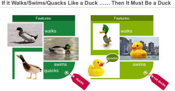
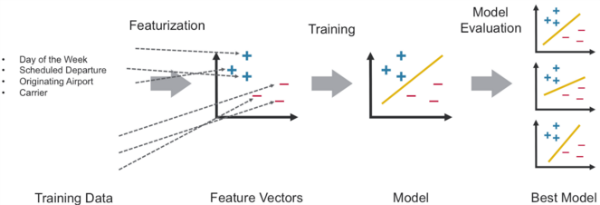
Classification is a family of supervised machine learning algorithms that identify which category an item belongs to (for example, whether a cancer tissue observation is malignant or not), based on labeled examples of known items (for example, observations known to be malignant or not). Classification takes a set of data with known labels and pre-determined features and learns how to label new records based on that information. Features are the “if questions” that you ask. The label is the answer to those questions. In the example below, if it walks, swims, and quacks like a duck, then the label is “duck.”
Let’s go through an example of Cancer Tissue Observations:
- What are we trying to predict?
- Whether a sample observation is malignant or not.
- This is the Label: malignant or not.
- What are the “if questions” or properties that you can use to predict?
- Tissue sample characteristics: Clump Thickness, Uniformity of Cell Size, Uniformity of Cell Shape, Marginal Adhesion, Single Epithelial Cell Size, Bare Nuclei, Bland Chromatin, Normal Nucleoli, Mitoses.
- These are the Features. To build a classifier model, you extract the features of interest that most contribute to the classification.
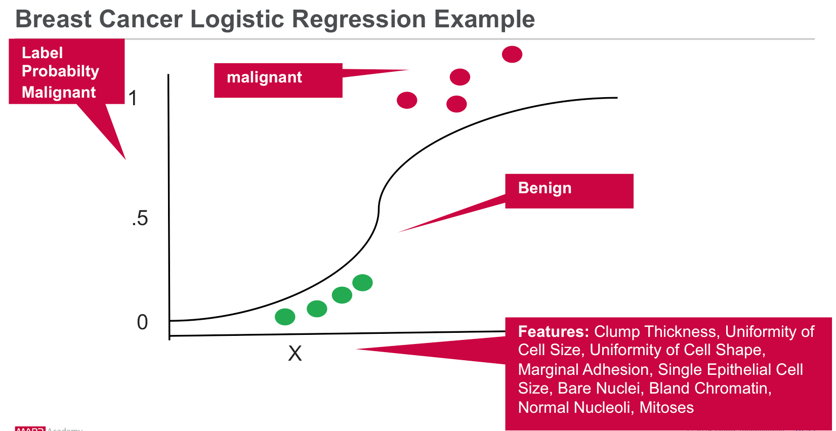
Logistic Regression
Logistic regression is a popular method to predict a binary response. It is a special case of Generalized Linear models that predicts the probability of the outcome. Logistic regression measures the relationship between the Y “Label” and the X “Features” by estimating probabilities using a logistic function. The model predicts a probability which is used to predict the label class.
Analyze Cancer Observations with Spark Machine Learning Scenario
Our data is from the Wisconsin Diagnostic Breast Cancer (WDBC) Data Set which categorizes breast tumor cases as either benign or malignant based on 9 features to predict the diagnosis. For each cancer observation, we have the following information:
1. Sample code number: id number
2. Clump Thickness: 1 - 10
3. Uniformity of Cell Size: 1 - 10
4. Uniformity of Cell Shape: 1 - 10
5. Marginal Adhesion: 1 - 10
6. Single Epithelial Cell Size: 1 - 10
7. Bare Nuclei: 1 - 10
8. Bland Chromatin: 1 - 10
9. Normal Nucleoli: 1 - 10
10. Mitoses: 1 - 10
11. Class: (2 for benign, 4 for malignant)
The Cancer Observation csv file has the following format :
1000025,5,1,1,1,2,1,3,1,1,2
1002945,5,4,4,5,7,10,3,2,1,2
1015425,3,1,1,1,2,2,3,1,1,2
In this scenario, we will build a logistic regression model to predict the label / classification of malignant or not based on the following features:
- Label → malignant or benign (1 or 0)
- Features → {Clump Thickness, Uniformity of Cell Size, Uniformity of Cell Shape, Marginal Adhesion, Single Epithelial Cell Size, Bare Nuclei, Bland Chromatin, Normal Nucleoli, Mitoses }
Spark ML provides a uniform set of high-level APIs built on top of DataFrames. The main concepts in Spark ML are:
- DataFrame: The ML API uses DataFrames from Spark SQL as an ML dataset.
- Transformer: A Transformer is an algorithm which transforms one DataFrame into another DataFrame. For example, turning a DataFrame with features into a DataFrame with predictions.
- Estimator: An Estimator is an algorithm which can be fit on a DataFrame to produce a Transformer. For example, training/tuning on a DataFrame and producing a model.
- Pipeline: A Pipeline chains multiple Transformers and Estimators together to specify a ML workflow.
- ParamMaps: Parameters to choose from, sometimes called a “parameter grid” to search over.
- Evaluator: Metric to measure how well a fitted Model does on held-out test data.
- CrossValidator: Identifies the best ParamMap and re-fits the Estimator using the best ParamMap and the entire dataset.
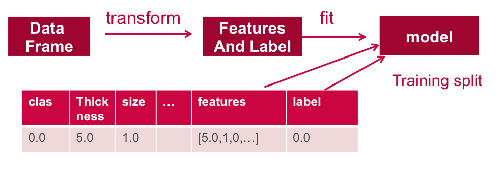
In this example, will use the Spark ML workflow shown below: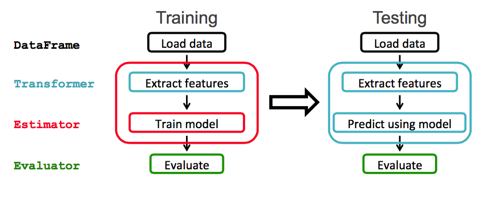
Software
This tutorial will run on Spark 1.6.1
- You can download the code and data to run these examples from here: https://github.com/caroljmcdonald/spark-ml-lr-cancer
- The examples in this post can be run in the Spark shell, after launching with the spark-shell command.
- You can also run the code as a standalone application as described in the tutorial on Getting Started with Spark on MapR Sandbox.
Log into the MapR Sandbox, as explained in Getting Started with Spark on MapR Sandbox, using userid user01, password mapr. Copy the sample data file to your sandbox home directory /user/user01 using scp. (Note you may have to update the Spark version on you Sandbox) Start the Spark shell with:
$spark-shell --master local[1]
Load and Parse the Data from a csv File
First, we will import the machine learning packages.
(In the code boxes, comments are in Green and output is in Blue)
import org.apache.spark._
import org.apache.spark.rdd.RDD
import org.apache.spark.sql.SQLContext
import org.apache.spark.ml.feature.StringIndexer
import org.apache.spark.ml.feature.VectorAssembler
import org.apache.spark.ml.classification.BinaryLogisticRegressionSummary
import org.apache.spark.ml.evaluation.BinaryClassificationEvaluator
import org.apache.spark.ml.classification.LogisticRegression
import org.apache.spark.ml.feature.StringIndexer
import org.apache.spark.ml.feature.VectorAssembler
import sqlContext.implicits._
import sqlContext._
import org.apache.spark.sql.functions._
import org.apache.spark.mllib.linalg.DenseVector
import org.apache.spark.mllib.evaluation.BinaryClassificationMetrics
We use a Scala case class to define the schema corresponding to a line in the csv data file.
// define the Cancer Observation Schema
case class Obs(clas: Double, thickness: Double, size: Double, shape: Double, madh: Double, epsize: Double, bnuc: Double, bchrom: Double, nNuc: Double, mit: Double)
The functions below parse a line from the data file into the Cancer Observation class.
// function to create a Obs class from an Array of Double.Class Malignant 4 is changed to 1
def parseObs(line: Array[Double]): Obs = {
    Obs(
      if (line(9) == 4.0) 1 else 0, line(0), line(1), line(2), line(3), line(4), line(5), line(6), line(7), line(8)
    )
}
// function to transform an RDD of Strings into an RDD of Double, filter lines with ?, remove first column
def parseRDD(rdd: RDD[String]): RDD[Array[Double]] = {
    rdd.map(_.split(",")).filter(_(6) != "?").map(_.drop(1)).map(_.map(_.toDouble))
}
Below we load the data from the csv file into an RDD of Strings. Then we use the map transformation on the rdd, which will apply the ParseRDD function to transform each String element in the RDD into an Array of Double. Then we use another map transformation, which will apply the ParseObs function to transform each Array of Double in the RDD into an Array of Cancer Observation objects. The toDF() method transforms the RDD of Array[[Cancer Observation]] into a Dataframe with the Cancer Observation class schema.
// load the data into a DataFrame
val rdd = sc.textFile("data/breast_cancer_wisconsin_data.txt")
val obsRDD = parseRDD(rdd).map(parseObs)
val obsDF = obsRDD.toDF().cache()
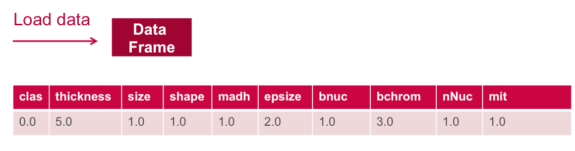
obsDF.registerTempTable("obs")DataFrame printSchema() Prints the schema to the console in a tree format
// Return the schema of this DataFrame
obsDF.printSchema

root
 |-- clas: double (nullable = false)
 |-- thickness: double (nullable = false)
 |-- size: double (nullable = false)
 |-- shape: double (nullable = false)
 |-- madh: double (nullable = false)
 |-- epsize: double (nullable = false)
 |-- bnuc: double (nullable = false)
 |-- bchrom: double (nullable = false)
 |-- nNuc: double (nullable = false)
 |-- mit: double (nullable = false)

// Display the top 20 rows of DataFrame
obsDF.show


+----+---------+----+-----+----+------+----+------+----+---+
|clas|thickness|size|shape|madh|epsize|bnuc|bchrom|nNuc|mit|
+----+---------+----+-----+----+------+----+------+----+---+
| 0.0|      5.0| 1.0|  1.0| 1.0|   2.0| 1.0|   3.0| 1.0|1.0|
| 0.0|      5.0| 4.0|  4.0| 5.0|   7.0|10.0|   3.0| 2.0|1.0|
| 0.0|      3.0| 1.0|  1.0| 1.0|   2.0| 2.0|   3.0| 1.0|1.0|
...
+----+---------+----+-----+----+------+----+------+----+---+
only showing top 20 rows
After a DataFrame is instantiated, you can query it using SQL queries. Here are some example queries using the Scala DataFrame API:
describe computes statistics for thickness column, including count, mean, stddev, min, and max
//  computes statistics for thickness
obsDF.describe("thickness").show

+-------+------------------+
|summary|         thickness|
+-------+------------------+
|  count|               683|
|   mean|  4.44216691068814|
| stddev|2.8207613188371288|
|    min|               1.0|
|    max|              10.0|
+-------+------------------+


// compute the avg thickness, size, shape grouped by clas (malignant or not)
sqlContext.sql("SELECT clas, avg(thickness) as avgthickness, avg(size) as avgsize, avg(shape) as avgshape FROM obs GROUP BY clas ").show

+----+-----------------+------------------+------------------+
|clas|     avgthickness|           avgsize|          avgshape|
+----+-----------------+------------------+------------------+
| 1.0|7.188284518828452| 6.577405857740586| 6.560669456066946|
| 0.0|2.963963963963964|1.3063063063063063|1.4144144144144144|
+----+-----------------+------------------+------------------+

// compute avg thickness grouped by clas (malignant or not)
obsDF.groupBy("clas").avg("thickness").show

+----+-----------------+
|clas|   avg(thickness)|
+----+-----------------+
| 1.0|7.188284518828452|
| 0.0|2.963963963963964|
+----+-----------------+
Extract Features
To build a classifier model, you first extract the features that most contribute to the classification. In the cancer data set, the data is labeled with two classes – 1 (malignant) and 0 (not malignant).
The features for each item consists of the fields shown below:
- Label → malignant: 0 or 1
- Features → {“thickness”, “size”, “shape”, “madh”, “epsize”, “bnuc”, “bchrom”, “nNuc”, “mit”}
Define Features Array
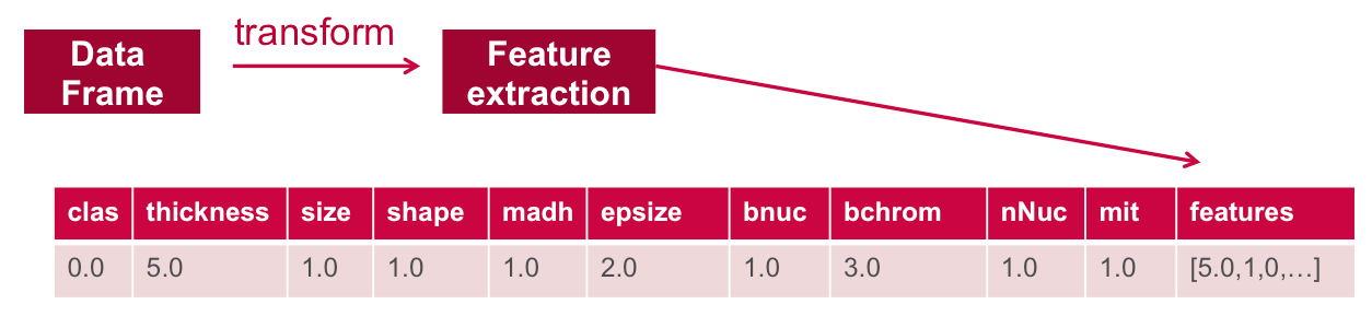
In order for the features to be used by a machine learning algorithm, the features are transformed and put into Feature Vectors, which are vectors of numbers representing the value for each feature.
Below a VectorAssembler is used to transform and return a new DataFrame with all of the feature columns in a vector column
//define the feature columns to put in the feature vector
val featureCols = Array("thickness", "size", "shape", "madh", "epsize", "bnuc", "bchrom", "nNuc", "mit")
//set the input and output column names
val assembler = new VectorAssembler().setInputCols(featureCols).setOutputCol("features")
//return a dataframe with all of the feature columns in a vector column
val df2 = assembler.transform(obsDF)
// the transform method produced a new column: features.
df2.show
+----+---------+----+-----+----+------+----+------+----+---+--------------------+
|clas|thickness|size|shape|madh|epsize|bnuc|bchrom|nNuc|mit| features|
+----+---------+----+-----+----+------+----+------+----+---+--------------------+
| 0.0| 5.0| 1.0| 1.0| 1.0| 2.0| 1.0| 3.0| 1.0|1.0|[5.0,1.0,1.0,1.0,...|
| 0.0| 5.0| 4.0| 4.0| 5.0| 7.0|10.0| 3.0| 2.0|1.0|[5.0,4.0,4.0,5.0,...|
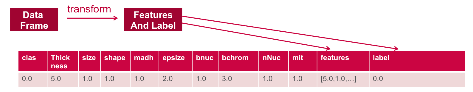
| 1.0| 8.0|10.0| 10.0| 8.0| 7.0|10.0| 9.0| 7.0|1.0|[8.0,10.0,10.0,8....|Next, we use a StringIndexer to return a Dataframe with the clas (malignant or not) column added as a label .
// Create a label column with the StringIndexer
val labelIndexer = new StringIndexer().setInputCol("clas").setOutputCol("label")
val df3 = labelIndexer.fit(df2).transform(df2)
// the transform method produced a new column: label.
df3.show
+----+---------+----+-----+----+------+----+------+----+---+--------------------+-----+
|clas|thickness|size|shape|madh|epsize|bnuc|bchrom|nNuc|mit| features|label|
+----+---------+----+-----+----+------+----+------+----+---+--------------------+-----+
| 0.0| 5.0| 1.0| 1.0| 1.0| 2.0| 1.0| 3.0| 1.0|1.0|[5.0,1.0,1.0,1.0,...| 0.0|
| 0.0| 5.0| 4.0| 4.0| 5.0| 7.0|10.0| 3.0| 2.0|1.0|[5.0,4.0,4.0,5.0,...| 0.0|
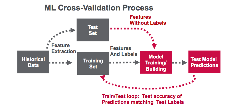
| 0.0| 3.0| 1.0| 1.0| 1.0| 2.0| 2.0| 3.0| 1.0|1.0|[3.0,1.0,1.0,1.0,...| 0.0|Below the data. It is split into a training data set and a test data set. 70% of the data is used to train the model, and 30% will be used for testing.
//  split the dataframe into training and test data
val splitSeed = 5043
val Array(trainingData, testData) = df3.randomSplit(Array(0.7, 0.3), splitSeed)
Train the Model
Next, we train the logistic regression model with elastic net regularization
The model is trained by making associations between the input features and the labeled output associated with those features.
// create the classifier,  set parameters for training
val lr = new LogisticRegression().setMaxIter(10).setRegParam(0.3).setElasticNetParam(0.8)
//  use logistic regression to train (fit) the model with the training data
val model = lr.fit(trainingData)

// Print the coefficients and intercept for logistic regression
println(s"Coefficients: ${model.coefficients} Intercept: ${model.intercept}")


Coefficients: (9,[1,2,5,6],[0.06503554553146387,0.07181362361391264,0.07583963853124673,0.0012675057388232965]) Intercept: -1.39319142312609
Test the Model
Next we use the test data to get predictions.
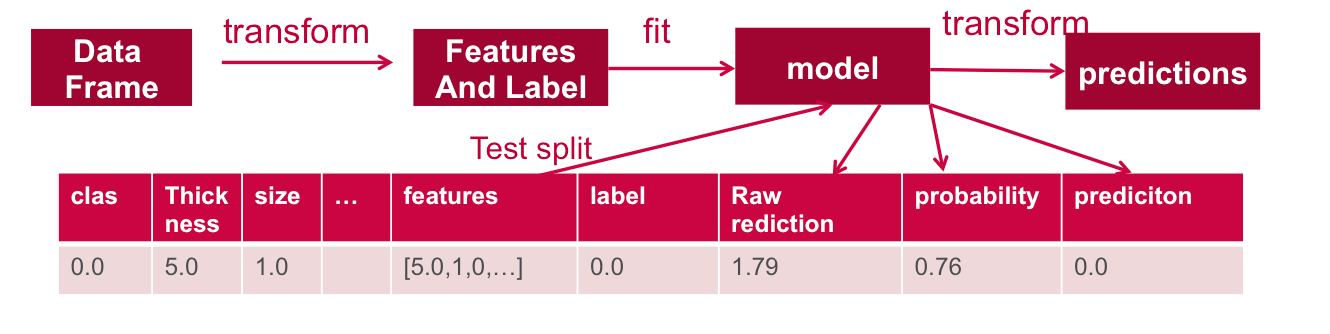
// run the  model on test features to get predictions
val predictions = model.transform(testData)
//As you can see, the previous model transform produced a new columns: rawPrediction, probablity and prediction.
predictions.show

+----+---------+----+-----+----+------+----+------+----+---+--------------------+-----+--------------------+--------------------+----------+
|clas|thickness|size|shape|madh|epsize|bnuc|bchrom|nNuc|mit|            features|label|       rawPrediction|         probability|prediction|
+----+---------+----+-----+----+------+----+------+----+---+--------------------+-----+--------------------+--------------------+----------+
| 0.0|      1.0| 1.0|  1.0| 1.0|   1.0| 1.0|   1.0| 3.0|1.0|[1.0,1.0,1.0,1.0,...|  0.0|[1.17923510971064...|[0.76481024658406...|       0.0|
| 0.0|      1.0| 1.0|  1.0| 1.0|   1.0| 1.0|   3.0| 1.0|1.0|[1.0,1.0,1.0,1.0,...|  0.0|[1.17670009823299...|[0.76435395397908...|       0.0|
| 0.0|      1.0| 1.0|  1.0| 1.0|   1.0| 1.0|   3.0| 1.0|1.0|[1.0,1.0,1.0,1.0,...|  0.0|[1.17670009823299...|[0.76435395397908...|       0.0|
| 0.0|      1.0| 1.0|  1.0| 1.0|   2.0| 1.0|   1.0| 1.0|1.0|[1.0,1.0,1.0,1.0,...|  0.0|[1.17923510971064...|[0.76481024658406...|       0.0|
| 0.0|      1.0| 1.0|  1.0| 1.0|   2.0| 1.0|   2.0| 1.0|1.0|[1.0,1.0,1.0,1.0,...|  0.0|[1.17796760397182...|[0.76458217679258...|       0.0|
+----+---------+----+-----+----+------+----+------+----+---+--------------------+-----+--------------------+--------------------+----------+
Below we evaluate the predictions, we use a BinaryClassificationEvaluator which returns a precision metric by comparing the test label column with the test prediction column. In this case, the evaluation returns 99% precision.
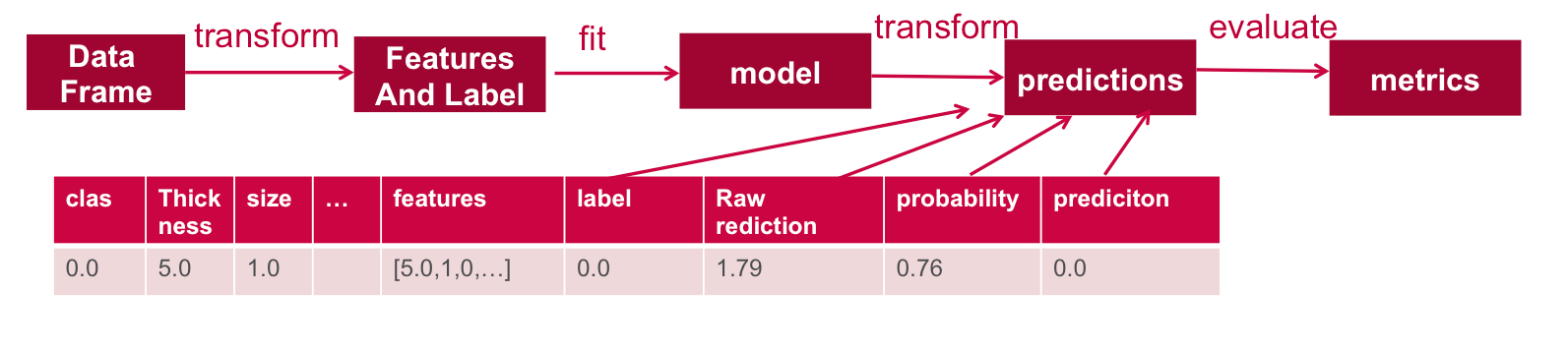
//A common metric used for logistic regression is area under the ROC curve (AUC). We can use the BinaryClasssificationEvaluator to obtain the AUC
// create an Evaluator for binary classification, which expects two input columns: rawPrediction and label.
val evaluator = new BinaryClassificationEvaluator().setLabelCol("label").setRawPredictionCol("rawPrediction").setMetricName("areaUnderROC")
// Evaluates predictions and returns a scalar metric areaUnderROC(larger is better).
val accuracy = evaluator.evaluate(predictions)
accuracy: Double = 0.9926910299003322
Below we calculate some more metrics. The number of false and true positive and negative predictions is also useful:
- True positives are how often the model correctly predicted a tumour was malignant
- False positives are how often the model predicted a tumour was malignant when it was benign
- True negatives indicate how the model correctly predicted a tumour was benign
- False negatives indicate how often the model predicted a tumour was benign when in fact it was malignant
// Calculate Metrics
val lp = predictions.select( "label", "prediction")
val counttotal = predictions.count()
val correct = lp.filter($"label" === $"prediction").count()
val wrong = lp.filter(not($"label" === $"prediction")).count()
val truep = lp.filter($"prediction" === 0.0).filter($"label" === $"prediction").count()
val falseN = lp.filter($"prediction" === 0.0).filter(not($"label" === $"prediction")).count()
val falseP = lp.filter($"prediction" === 1.0).filter(not($"label" === $"prediction")).count()
val ratioWrong=wrong.toDouble/counttotal.toDouble
val ratioCorrect=correct.toDouble/counttotal.toDouble


counttotal: Long = 199
correct: Long = 168
wrong: Long = 31
truep: Long = 128
falseN: Long = 30
falseP: Long = 1
ratioWrong: Double = 0.15577889447236182
ratioCorrect: Double = 0.8442211055276382


// use MLlib to evaluate, convert DF to RDD
val  predictionAndLabels =predictions.select("rawPrediction", "label").rdd.map(x => (x(0).asInstanceOf[DenseVector](1), x(1).asInstanceOf[Double]))
val metrics = new BinaryClassificationMetrics(predictionAndLabels)
println("area under the precision-recall curve: " + metrics.areaUnderPR)
println("area under the receiver operating characteristic (ROC) curve : " + metrics.areaUnderROC)
// A Precision-Recall curve plots (precision, recall) points for different threshold values, while a receiver operating characteristic, or ROC, curve plots (recall, false positive rate) points. The closer  the area Under ROC is to 1, the better the model is making predictions.

area under the precision-recall curve: 0.9828385182615946
area under the receiver operating characteristic (ROC) curve : 0.9926910299003322
Want to learn more?
- Free On Demand Apache Spark Training
- MapR and Spark
- Apache Spark ML overview
- Apache Spark ML Logistic Regression
- Artificial Intelligence Reads Mammograms With 99% Accuracy
In this blog post, we showed you how to get started using Apache Spark’s machine learning Logistic Regression for classification. If you have any further questions about this tutorial, please ask them in the comments section below.
| Reference: | Predicting Breast Cancer Using Apache Spark Machine Learning Logistic Regression from our JCG partner Carol McDonald at the Mapr blog. |
