Distributed Data Analysis with Docker Swarm

Florian MotlikApril 8th, 2016Last Updated: April 8th, 2016

0 28 10 minutes read

The purpose of this post is to show how powerful and flexible Docker Swarm can be when combined with standard UNIX tools to analyze data in a distributed fashion. To do this, let’s write a simple MapReduce implementation in bash/sh that uses Docker Swarm to schedule Map jobs on nodes across the cluster.

MapReduce is usually implemented when there’s a large dataset to process. For the sake of simplicity and for reproducibility by the reader, we’re using a very small dataset composed of a few megabytes of text files.

This post is not about showing you how to write a MapReduce program. It’s also not about suggesting that MapReduce is best done in this way. Instead, this post is about making you aware that the plain old UNIX tools such as sort, awk, netcat, pv, uniq, xargs, pipe, join, time, and cat can be useful for distributed data processing when running on top of a Docker Swarm cluster.

Because this is only an example, there’s a lot of work to do to gain fault tolerance resilience and redundancy. A solution like the one proposed here can be useful if you happen to have a one-time use case and you don’t want to invest time in something more complicated like Hadoop. If you have a frequent use case, I recommend you use Hadoop instead.

Requirements for Our MapReduce Implementation with Docker Swarm

To reproduce the examples in this post, you’re going to need a few things:

Docker installed on your local machine
A running Swarm cluster (if you don’t have one, don’t worry. I’ll explain how to obtain one for this purpose in a fast and easy way)
Docker Machine installed on your local machine (to set up the Swarm cluster if you don’t already have one)

MapReduce is a programming paradigm with the aim of processing large datasets in a distributed way on a cluster (in our case a Swarm cluster). As the name suggests, MapReduce is composed of two fundamental steps:

Map: The master node takes a large dataset and distributes it to compute nodes to perform analysis on. Each node returns a result.
Reduce: Gather the result of each Map and aggregate them to produce the final answer.

Setting up the Swarm cluster

If you already have a Swarm cluster, you can skip this section. Just ensure that you’re connecting to the Swarm cluster when using the Docker client. For this purpose, you can inspect the DOCKER_HOST environment variable.

I wrote a setup script so we can easily create a Swarm cluster on DigitalOcean. In order to use it, you need a DigitalOcean account and an API key to allow Docker Machine to manage instances for you. You can obtain the API key here.

When you are done with the API key, export it so it can be used in the setup script:

export DO_ACCESS_TOKEN=aa9399a2175a93b17b1c86c807e08d3fc4b79876545432a629602f61cf6ccd6b

Now we’re ready to write the create-cluster.sh script:

#!/bin/bash

# configuration
agents="agent1 agent2"

token=$(docker run --rm swarm create)

# Swarm manager machine
echo "Create swarm manager"
docker-machine create \
    -d digitalocean \
    --digitalocean-access-token=$DO_ACCESS_TOKEN \
    --swarm --swarm-master \
    --swarm-discovery token://$token \
    manager

# Swarm agents
for agent in $agents; do
    (
    echo "Creating ${agent}"

    docker-machine create \
        -d digitalocean \
        --digitalocean-access-token=$DO_ACCESS_TOKEN \
        --swarm \
        --swarm-discovery token://$token \
        $agent
    ) &
done
wait

# Information
echo ""
echo "CLUSTER INFORMATION"
echo "discovery token: ${token}"
echo "Environment variables to connect trough docker cli"
docker-machine env --swarm manager

As you can note, this script is composed of three parts:

configuration: Here you have two variables used to configure the entire cluster. The agents variable defines how many Swarm agents to put in the cluster while the token variable is populated with the swarm create command that generates a Docker Hub token used by your cluster for service discovery. If you don’t like the token approach, you can use your own discovery service like Consul, ZooKeeper, or Etcd.
Creation of the Swarm master machine: This is the machine that will expose the Docker Remote API via tcp.
Creation of the Swarm agent machines: According to the configuration, a machine will be created on DigitalOcean for each specified name agent1 agent2 and configured to join the cluster of the previously created Swarm manager.
Print information about the generated cluster: When machines are running, the script just prints informations about the generated cluster and how to connect to it with the Docker client.

Now we can finally execute the create-cluster.sh script:

chmod +x create_cluster.sh
./create_cluster.sh

After a few minutes and a few lines of output and if nothing went wrong, we should see something like this:

CLUSTER INFORMATION
discovery token: 9effe6d53fdec36e6237459313bf2eaa
Environment variables to connect trough docker cli
export DOCKER_TLS_VERIFY="1"
export DOCKER_HOST="tcp://104.236.46.188:3376"
export DOCKER_CERT_PATH="/home/fntlnz/.docker/machine/machines/manager"
export DOCKER_MACHINE_NAME="manager"
# Run this command to configure your shell: 
# eval $(docker-machine env --swarm manager)

As suggested, you have to run the command to configure your shell in order to connect to the Swarm cluster Docker daemon.

eval $(docker-machine env --swarm manager)

To verify that the cluster is up and running, you can use:

docker-machine ls

which should print:

NAME      ACTIVE      DRIVER         STATE     URL                         SWARM              DOCKER    ERRORS
agent1    -           digitalocean   Running   tcp://104.236.26.148:2376   manager            v1.10.3   
agent2    -           digitalocean   Running   tcp://104.236.21.118:2376   manager            v1.10.3   
manager   * (swarm)   digitalocean   Running   tcp://104.236.46.188:2376   manager (master)   v1.10.3

Please note that the only one that has something under the ACTIVE column is the master. This is because you ran that eval command to configure your shell previously.

Collecting Data for Analysis

Data analysis would be nothing without data to be analyzed. We’re going to use a few transcripts of the latest seasons of the popular British sci-fi series Doctor Who. For this purpose, I created a Gist with a few of them taken from The Doctor Who Transcripts.

I actually added to the Gist only the most recent episodes (beginning in 2005) from the Ninth Doctor. You can obtain the transcripts by cloning my Gist:

git clone https://gist.github.com/fa9ed1ad11ba09bd87b2d25a14f65636.git who-transcripts

Once you’ve cloned the Gist, you should end up with a who-transcripts folder containing 130 transcripts.

Since one of our requirements for this post is that data analysis be done with UNIX tools, we can use AWK for the map program.

In order to be useful for the reduce step, our map program should be able to transform a transcript like this:

[Albion hospital]
(The patients are almost within touching distance.) 
DOCTOR: Go to your room. 
(The patients in the ward and the child in the house stand still.) 
DOCTOR: Go to your room. I mean it. I'm very, very angry with you. I am very, very cross. Go to your room! 
(The child and the patients hang their heads in shame and shuffle away. The child leaves the Lloyd's house and the patients get back into bed.) 
DOCTOR: I'm really glad that worked. Those would have been terrible last words.

[The Lloyd's dining room]

In a key, value pair like this:

DOCTOR go
DOCTOR to
DOCTOR your
DOCTOR room
DOCTOR Im
DOCTOR really
DOCTOR glad
...

To do that, Map has to skip lines that are not in the format <speaker>: <phrase>, and then for each word it has to print the speaker name and the word itself.

For this purpose, we can write a simple AWK program such as map.awk:

#!/usr/bin/awk -f
{
    if ($0 ~ /^(\w+)(.\[\w+\])?:/) {
        split ($0, line, ":");
        character=line[1];
        phrase=tolower(gensub(/[^a-zA-Z0-9 ]/, "", "g", line[2]));
        count=split(phrase, words, " ");
        for (i = 0; ++i <= count;) {
            print  character " " words[i]
        }
    }
}

On your local machine, you can easily try the map program with:

cat who-transcripts/27-1.txt | ./map.awk

Scheduling Map Jobs

Now that we have our Map program, we can think about how to start scheduling map jobs on our cluster. Our scheduler will be in charge of:

Managing how many jobs can be done simultaneously
Copying the map program into executors
Telling the executor to run map programs
Copying the data to executors
Running the map program and joining each single executor’s result with the others
Garbage collecting containers not needed anymore

For this purpose, we can write a bash script that reads all the transcripts from the who-transcripts folder. It will also use the Docker client to connect to the Swarm cluster and do all the magic!

A script like the one below can accomplish this important task:

#!/bin/bash

function usage {
    echo "USAGE: "
    echo "    ./scheduler.sh <transcripts folder> <max concurrent jobs>"
}

# Argument checking
transcripts_folder=$1

if [ -z "$1" ]; then
    echo "Please provide a folder from which take transcripts"
    echo ""
    usage
    exit 1
fi

if [ ! -d "$transcripts_folder" ]; then
    echo "Please provide a valid folder from which take transcripts"
    echo ""
    usage
    exit 1
fi
maxprocs=$2
if [ -z "$2" ]; then
    maxprocs=5
fi

# Scheduling
proc=0
seed=`uuidgen`

# Cycle trough transcripts and start jobs
for transcript in $transcripts_folder/*; do
    (container=`docker run --name "${seed}.$proc" -d  alpine sh -c "while true; do sleep 5; done"` > /dev/null
    echo "[MAP] transcript: ${transcript} => container: ${container}"
    docker cp map.awk $container:/map
    cat $transcript | docker exec -i $container ./map >> result.txt
    docker rm -f $container > /dev/null) &
    (( proc++%maxprocs==0 )) && wait;
done

# Remove containers
docker ps -aq --filter "name=$1" | xargs docker rm -f

The script is made of three important parts:

Argument Checking: The sole purpose of this part is to retrieve and check the needed arguments for jobs execution.
Jobs Execution: This part consists of a for loop that iterates trough transcript files in the provided folder. On each iteration, a container is started, and the map.awk script is copied to it just before being executed. The output of the mapping is redirected to the result.txt file which collects all mapping outputs. The for loop is controlled by the maxprocs variable that determines the maximum number of concurrent jobs.
Containers removal: Used containers should be removed during the for loop; if that doesn’t happen, they are removed after the loop ends.

The scheduler script could be simplified by running the container with the -rm option, but that would require for the map.awk script to be already inside the image before running.

Since the scheduler is capable of transferring needed data to executors, we don’t need anything else, and we can run the scheduler. But before running the scheduler, we have to tell the Docker client to connect to the Swarm cluster instead of the local engine.

eval $(docker-machine env --swarm manager)

This will start the scheduler using the who-transcripts folder with 40 as the maximum number of concurrent jobs.

./scheduler.sh who-transcripts 40

While executing, the scheduler should output something similar:

[MAP] transcript: who-transcripts/27-10.txt => container: f1b4bdf37b327d6d3c288cc1e6ce1b7f274b3712bc54e4315d24a9524801b230
[MAP] transcript: who-transcripts/27-12.txt => container: 03e18bf08f923c0b52121a61f1871761bf516fe5bc53140da7fa08a9bcb9294c
[MAP] transcript: who-transcripts/27-11.txt => container: dadfb0e2cccf737198e354d2468bdf3eb8419ec131ed8a3852eca53f1e57314b
[MAP] transcript: who-transcripts/27-2.txt => container: 69bb0eb07df7a356d10add9d466f7d6e2c8b7ed246ed9922dc938c0f7b4ee238
[MAP] transcript: who-transcripts/28-1.txt => container: 3f56522aac45fd76f88a190611fb6e3f96f4a65e79e8862f7817be104f648737
[MAP] transcript: who-transcripts/28-6.txt => container: 05048e807996b63231c59942a23f8504eab39ece32e616644ccef2de7cb01d5c
[MAP] transcript: who-transcripts/28-0.txt => container: a0199b5d64ca012e411da09d85081a604f87500f01e193395828e7911f045075

When the scheduler completes, we can inspect the result.txt file . Here’s the first 20 lines:

DOCTOR go
DOCTOR to
DOCTOR your
DOCTOR room
DOCTOR go
DOCTOR to
DOCTOR your
DOCTOR room
DOCTOR i
DOCTOR mean
MICKEY it
ROSE im
DOCTOR very
DOCTOR very
DOCTOR angry
DOCTOR with
MICKEY you
DOCTOR i
DOCTOR am
ROSE very

Great! That’s a key, value <name> <sentence>. So let’s see if we can reduce this data to something useful with this data with a UNIX command:

cat result.txt | sort | uniq -c | sort -fr

The above reduction command sorts the file, filters unique rows, and then sorts them again in reverse order so that the most common words by speaker are shown first. The output of the first 20 lines of this command then is:

9271 DOCTOR the
   7728 DOCTOR you
   5290 DOCTOR a
   5219 DOCTOR i
   4928 DOCTOR to
   3959 DOCTOR it
   3501 DOCTOR and
   3476 DOCTOR of
   2595 DOCTOR that
   2457 DOCTOR in
   2316 DOCTOR no
   2309 DOCTOR its
   2235 DOCTOR is
   2150 DOCTOR what
   2088 DOCTOR this
   2009 DOCTOR me
   1865 DOCTOR on
   1681 DOCTOR not
   1580 DOCTOR just
   1531 DOCTOR im

This means that the most common word said by the Doctor is the. Here’s the distribution graph of the 50 most used words:

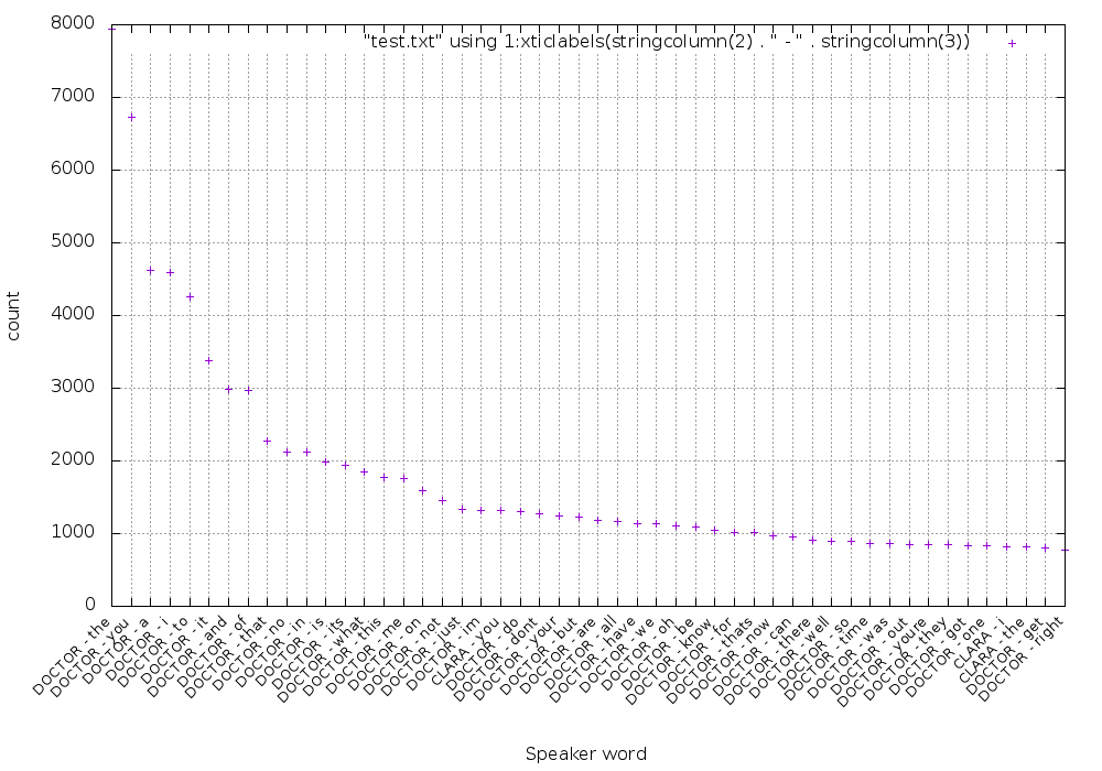
If you’re interested, I generated this graph using this gnuplot script:

reset
set term png truecolor size 1000,700
set output "dist.png"
set xlabel "Speaker word"
set ylabel "count"
set grid
set boxwidth 0.95 relative
set style fill transparent solid 0.5 noborder
set xtics rotate by 45 right
set xtics font ", 10"
plot "result.txt" using 1:xticlabels(stringcolumn(2) . " - " . stringcolumn(3))

Let’s try something more meaningful — let’s look at how often the word tardis has been said:

cat result.txt | sort | uniq -c | sort -fr | grep 'tardis'

As expected, this shows that the Doctor is the one who talks about the “TARDIS” most of all:

335 DOCTOR tardis
     43 CLARA tardis
     22 ROSE tardis
     22 AMY tardis
     18 RIVER tardis
     16 RORY tardis
     10 DOCTOR [OC] tardis
      9 MICKEY tardis
      8 MARTHA tardis
      6 IDRIS tardis
      6 DOCTOR tardises
      5 JACK tardis
      5 DONNA tardis
      4 MASTER tardis
      4 DALEK tardis
      3 TASHA tardis
      3 MARTHA [OC] tardis
      3 KATE tardis
      3 DOCTOR [memory] tardis
      2 RIVER [OC] tardis
      2 MOMENT tardis
      2 MISSY tardis
      2 DALEKS [OC] tardis
      1 YVONNE tardis
      1 WHITE tardis
      1 VICTORIA tardis
      1 VASTRA tardis
      1 UNCLE tardises
      1 SUSAN [OC] tardis
      1 SEC tardis
      1 SARAH tardis
      1 ROSITA tardis
      1 RORY [OC] tardis
      1 ROBIN tardis
      1 OSGOOD tardis
      1 MOTHER tardis
      1 MACE tardis
      1 LAKE tardis
      1 KATE tardisproofed
      1 K9 tardis
      1 JENNY tardis
      1 JACKIE tardis
      1 IDRIS tardises
      1 HOWIE tardis
      1 HOUSE [OC] tardises
      1 HOUSE [OC] tardis
      1 HANDLES tardis
      1 GREGOR tardis
      1 FABIAN tardis
      1 EDITOR tardis
      1 DOCTOR tardisll
      1 DAVROS tardis
      1 DANNY tardis
      1 DALEK [OC] tardis
      1 CRAIG tardis
      1 CLARK tardis
      1 CLARA [OC] tardis
      1 BORS tardis
      1 BOB [OC] tardis
      1 BLUE tardis
      1 AUNTIE tardis
      1 ASHILDR tardis

Conclusion

Docker Swarm is a very flexible tool, and UNIX philosophy is more relevant than ever when performing data analysis. Here we showed how a simple task can be distributed on a cluster by mixing Swarm with a few commands — a possible evolution of this is using a more maintainable approach.

A few possible improvements could be:

Use a real programming language instead of AWK and Bash scripts.
Build and push a Docker image featuring all the needed programs (instead of copying them into Alpine on Docker run).
Put data closest to where it’s being processed (in the example, we loaded the data into the cluster at runtime with the scheduler).
Last but not least: Keep in mind that if you start having frequent and more complicated use cases, Hadoop is your friend.

Reference:

Distributed Data Analysis with Docker Swarm from our JCG partner Lorenzo Fontana at the Codeship Blog blog.