Processing real-time data with Storm, Kafka and ElasticSearch – Part 1

Ioannis KostarasOctober 21st, 2020Last Updated: October 21st, 2020

2 339 12 minutes read

This is an article of processing real-time data with Storm, Kafka and ElasticSearch.

1. Introduction

How would you process a stream of real or near-real time data?

In the era of Big Data, there are a number of technologies available that can help you in this task. In this series of articles we shall see a real example scenario and investigate the available technologies.

1. Introduction

2. Example data and scenario

3. ElasticSearch

3.1. Install ElasticSearch

4. Summary

5. References

Let’s first see some definitions first.

Big data is best understood by considering four different properties: volume, velocity, variety, and veracity.

Volume: enormous amounts of data
Velocity: the rate at which data is produced; deals with the pace at which data flows into a system, both in terms of the amount of data and the fact that it’s a continuous flow of data.
Variety: Any type of data – structured and unstructured
Veracity: the accuracy of incoming and outgoing data

Different big data tools exist that serve different purposes:

Data processing tools perform some form of calculation to the data
Data transfer tools gather and ingest data into the data processing tools
Data storage tools store data during various processing stages

Data processing tools can be further categorised into:

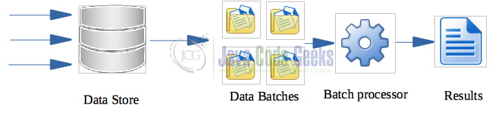
Batch processing: a batch is a collection of data to be processed together (see Figure 1). Batch processing allows you to join, merge, or aggregate different data points together. Its results are usually not available until the entire batch has completed processing. The larger your batch, the longer you have to wait to get useful information from it. If more immediate results are required, stream processing is a better solution.
Stream processing: A stream processor acts on an unbounded stream of data instead of a batch of data points that is being ingesting continuously (a “stream”) (see Figure 2). Unlike a batch process, there’s no well-defined beginning or end to the data points flowing through this stream; it’s continuous. Low latency (or high velocity) is the keyword here for choosing stream processing.

2. Example data and scenario

We are going to build a DRS or Data Reduction System using some realistic data. According to wikipedia, “Data reduction is the transformation of numerical or alphabetical digital information … into a corrected, ordered, and simplified form. The basic concept is the reduction of multitudinous amounts of data down to the meaningful parts.”

The data sources will be actual historic flight data which you can download freely from here. Data Field Descriptions are also available but you don’t need to understand all of them in order to be able to follow these articles. Our final target is to be able to display the flight historical data on a map.

Before we proceed to an architecture of the solution, let’s briefly describe the most important fields that we will use (depending on how someone is going to use the data, different fields are more important than other in different use cases):

Rcvr (integer) – “Receiver ID number” which has the format RRRYXXX
Icao (six-digit hex) – the six-digit hexadecimal identifier broadcast by the aircraft over the air in order to identify itself.
FSeen (datetime – epoch format) – date and time the receiver first started seeing the aircraft on this flight.
Alt (integer) – The altitude in feet at standard pressure (broadcasted by the aircraft)
Lat (float) – The aircraft’s latitude over the ground.
Long (float) – The aircraft’s longitude over the ground.
Spd (knots, float) – The ground speed in knots.
SpdTyp (integer) – The type of speed that Spd represents. Only used with raw feeds. 0/missing = ground speed, 1 = ground speed reversing, 2 = indicated air speed, 3 = true air speed.
Year (integer) – The year that the aircraft was manufactured.
Mil (boolean) – True if the aircraft appears to be operated by the military. Based on certain range of ICAO hex codes that the aircraft broadcasts.
Cou (string) – The country that the aircraft is registered to. Based on the ICAO hex code range the aircraft is broadcasting.
Gnd (boolean) – True if the aircraft is on the ground. Broadcast by transponder.
Call (alphanumeric) – The callsign of the aircraft.
CallSus (boolean) – True if the callsign may not be correct. Based on a checksum of the data received over the air.

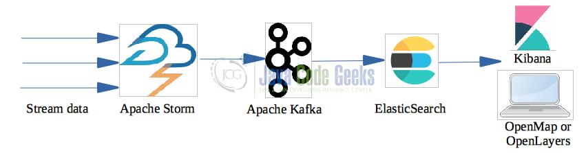
The final processing chain that we are going to build is shown in Figure 3:

Another stack of technologies that you could use instead is SMACK [1]:

Spark: The engine (alternative to Storm)
Mesos: The container
Akka: The model
Cassandra: The storage (alternative to ElasticSearch)
Kafka: The message broker

Or, you could try to implement it yourself in your favourite programming language (see Figure 4).

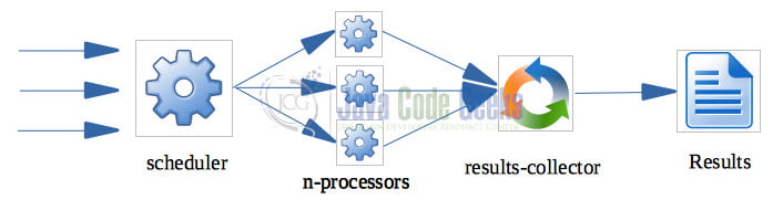
Figure 4. – Stream processing architecture

A single-threaded scheduler distributes the work to a number of processors (which could be arrays of Raspberry Pis for example) in a round-robin way, using e.g. MQTT for data exchange. Each processor processes the data in parallel and produces results which are gathered by a collector that is responsible for either storing them to a database, a NAS, or present them in real-time.

Since we don’t have any connection to a real sensor (e.g. radar) to receive real time flight data in order to demonstrate actual stream processing, we can only demonstrate batch processing (i.e. download the historic flight data and process them offline).

We will also go backwards. We will start by storing the data directly to ElasticSearch and visualise them in Kibana or in another UI application. In the following articles we will add Apache Storm and Apache Kafka into the game.

3. ElasticSearch

Elasticsearch is a distributed document-oriented search engine, which is used to store data in the form of documents. ElasticSearch is an open source real-time search engine which is platform independent (written in Java), distributed (can be scaled horizontally by adding new nodes to its cluster(s)) and can be easily integrated. In short, ElasticSearch is:

Scalable across multiple nodes (i.e. horizontally scalable)
performant (search results are very fast)
multilingual (you can search on your own native language)
document-oriented; stores the data in schema-less JSON format
supports auto-completion and instant search
supports fuzziness, i.e. small typos in search strings still returns valid results
open-source at no cost

ElasticStack consists of a number of products:

ElasticSearch, that we will focus in this article,
Kibana, an analytics and visualization platform, which lets you easily visualize data from Elasticsearch and analyze it to make sense of it. You can think of Kibana as an Elasticsearch dashboard where you can create visualizations, such as pie charts, line charts, etc. We will use Kibana to visualise our air traffic data. Kibana also provides an interface to manage certain parts of Elasticsearch, such as authentication and authorisation and a web interface to the data stored in ElasticSearch. It allows you to query ElasticSearch using a REST interface and displays the results.
LogStash, is a data processing pipeline. Traditionally it has been used to process logs from applications and send them to Elasticsearch, hence the name. The data that Logstash receives are handled as events that are processed by LogStash to be sent to various destinations, like ElasticSearch for example, but not only. A Logstash pipeline consists of three stages (which can use plugins): inputs, filters, and outputs. There are a lot of input plugins, so chances are that you will find what you need. An output plugin is where we send the processed events to (called stashes). A Logstash pipeline is defined in a proprietary markup format that is similar to JSON.
Beats, is a collection of so-called data shippers (called beats), i.e. lightweight agents with a single purpose that you install on servers, which then send data to Logstash or Elasticsearch. There are a number of beats that collect different kinds of data and serve different purposes. For example, Filebeat is used for collecting log files and sending the log entries off to either Logstash or Elasticsearch. Metricbeat collects system-level and/or service metrics (e.g. CPU and memory usage etc.). Heartbeat monitors a service’s uptime etc.
X-pack, is a pack of features that adds additional functionality to Elasticsearch and Kibana, like Security (authentication and authorisation), Performance (monitoring), Reporting, and Machine Learning. X-Pack also provides two useful modules called Graph (that finds the relevance in your data) and SQL (that allows to query ElasticSearch using SQL queries instead of using the Query DSL of ElasticSearch).

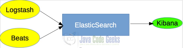
Putting the above together, ingesting data into Elasticsearch can be done with Beats and/or Logstash, but also directly via ElasticSearch’s API. Kibana is used to visualize the data from ElasticSearch.

Storm Kafka ElasticSearch - The Elastic Stack — Figure 5. – The Elastic Stack

Since this is going to be a long series of articles, in this article we shall learn how to install, start and stop ElasticSearch and Kibana. In the next article, we will provide an overview of the products and learn how to import batch flight data into ElasticSearch.

3.1 Install ElasticSearch & Kibana

Navigate to the ElasticSearch web site and download ElasticSearch for your platform. Once you unzip/untar it, you will see the following directory structure:

bin
config
data
jdk
lib
logs
modules
plugins

The main configuration file is config/elasticsearch.yml.

Execute ElasticSearch by typing:

cd <elasticsearch-installation>
bin/elasticsearch

and navigate with a browser to http://localhost:9200/. If you see something like the following, then congrats, you have a running instance of ElasticSearch in your machine, or node.

{
  "name" : "MacBook-Pro.local",
  "cluster_name" : "elasticsearch",
  "cluster_uuid" : "jyxqsR0HTOu__iUmi3m3eQ",
  "version" : {
    "number" : "7.9.0",
    "build_flavor" : "default",
    "build_type" : "tar",
    "build_hash" : "a479a2a7fce0389512d6a9361301708b92dff667",
    "build_date" : "2020-08-11T21:36:48.204330Z",
    "build_snapshot" : false,
    "lucene_version" : "8.6.0",
    "minimum_wire_compatibility_version" : "6.8.0",
    "minimum_index_compatibility_version" : "6.0.0-beta1"
  },
  "tagline" : "You Know, for Search"
}

ElasticSearch consists of a cluster of nodes (a.k.a. instances of ElasticSearch that store data). Each node stores parts of the data. You can run more than one instances in the same machine even though this is not recommended. My ElasticSearch instance cluster is called “elasticsearch” and consists of only one node, the instance I just started. You can run different clusters, too, even though, one cluster is usually enough. An ElasticSearch node will always be part of a cluster.

http://localhost:9200/_cluster/health?pretty

{
  "cluster_name" : "elasticsearch",
  "status" : "green",
  "timed_out" : false,
  "number_of_nodes" : 1,
  "number_of_data_nodes" : 1,
  "active_primary_shards" : 0,
  "active_shards" : 0,
  "relocating_shards" : 0,
  "initializing_shards" : 0,
  "unassigned_shards" : 0,
  "delayed_unassigned_shards" : 0,
  "number_of_pending_tasks" : 0,
  "number_of_in_flight_fetch" : 0,
  "task_max_waiting_in_queue_millis" : 0,
  "active_shards_percent_as_number" : 100.0
}

The cluster status is green and we see that it contains only 1 node.

Data are stored as JSON objects (or documents) in ElasticSearch. Documents are organised inside a cluster using indices. An index groups documents together logically, as well as provides configuration options related to scalability and availability. An index is a collection of documents that have similar characteristics and are logically related. E.g. we can have an index called Flight. Search queries run against indices.

Data are distributed in the various nodes. But how is this actually achieved? ElasticSearch uses sharding. Sharding is a way to divide an index into separate pieces, where each piece is called a shard. Sharding allows data to be scaled horizontally. E.g. imagine we have a cluster with two nodes, each of 1TB disk storage and an index of 1,2TB of data. Obviously, the index cannot be stored in any of the two nodes. ElasticSearch splits the data in two shards of 600 GB and stores each shard to a different node. (ElasticSearch can decide to create 4 shards etc.). A shard can store up to 2 billion documents. Queries can be distributed and parallelized across and index’s shards, thus improving search performance and throughput. The default number of shards per index is one, though, but this can change as data are increased/decreased.

But what happens if there is a disk failure and the node where a shard is stored breaks down? If we have only one node, then all data are lost. ElasticSearch supports shard replication for fault tolerance by default. Replica shards of the primary shards are created in nodes other than the node where the primary shard is stored. Both primary and replica shards are called a replication group. In our example where we only have one node, no replication takes place. If there is a disk failure, all my data are lost. The more nodes we add, the more the availability is increased by spreading shards around the nodes.

One can also create snapshots for backups, but a snapshot is a static view of the data at a moment in time. Snapshots can be useful when, for example, you wish to execute an update query to the data which you are not sure if it will succeed or corrupt the data. You take a snapshot before, and if the update fails, you rollback the data from the snapshot.

Replication can also increase the throughput of a given index. Like increasing the number of shards increases the throughput, increasing the number of replica shards has the same effect. So, if we have, for example, two replicas of a primary shard, ElasticSearch can handle three parallel queries of the same index at the same time.

Nodes can have different roles in ElasticSearch: master, data, ingest, machine learning (ml and xpack.ml), coordination, but this is outside the purpose of this article.

http://localhost:9200/_stats?pretty

{
  "_shards" : {
    "total" : 0,
    "successful" : 0,
    "failed" : 0
  },
  "_all" : {
    "primaries" : { },
    "total" : { }
  },
  "indices" : { }
}

An ElasticSearch cluster exposes a REST API to send commands to. The verbs, or commands, to use are typically GET, POST, PUT and DELETE.

There are a number of ways to issue commands to ElasticSearch.

by issuing the appropriate URL in either a browser or using the curl command
via Kibana’s Console Tool

Syntax for the curl command:

curl -X<VERB> '<PROTOCOL>://<HOST>:<PORT>/<PATH>?<QUERY_STRING>' -d '<BODY>'

<VERB> The appropriate HTTP method or verb. For example, GET, POST, PUT, HEAD, or DELETE.
<PROTOCOL> Either http or https. Use the latter if you have an HTTPS proxy in front of Elasticsearch or you use Elasticsearch security features to encrypt HTTP communications.
<HOST> The hostname of any node in your Elasticsearch cluster. Alternatively, use localhost for a node on your local machine.
<PORT> The port running the Elasticsearch HTTP service, which defaults to 9200.
<PATH> The API endpoint, which may contain multiple components, such as _cluster/stats or _nodes/stats/jvm.
<QUERY_STRING> Any optional query-string parameters. For example, ?pretty will pretty-print the JSON response to make it easier to read.
<BODY> A JSON-encoded request body (if necessary).

E.g.

curl -X GET "localhost:9200/flight/_doc/1?pretty"

will return all documents stored in the index flight. Since we haven’t inserted any documents in ElasticSearch yet, this query will return an error.

Via Kibana’s console. Download Kibana ,unzip/untar it to a folder and execute it by issuing the following commands:

cd <kibana-installation>
bin/kibana

Please make sure that ElasticSearch is already up and running before you start Kibana. Kibana’s directory structure is as follows:

bin
built_assets
config
data
node
node_modules
optimize
package.json
plugins
src
webpackShims
x-pack

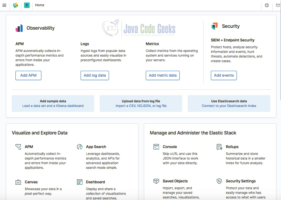
The first time you run Kibana (http://localhost:5601), you are requested to either try the provided sample data or explore your own. Make your choice. You can install the provided data in order to explore its capabilities.

You may access Kibana’s console from this URL:

http://localhost:5601/app/kibana#/dev_tools/console

or click on Console hyperlink from the Manage and Administer the Elastic Stack area or click on the Dev Tools icon from the vertical toolbar on the left side (it depends on the version of Kibana you are using).

Storm Kafka ElasticSearch - Kibana — Figure 6. – Kibana

Let’s issue the commands we sent above using the browser:

GET /_cluster/health?pretty
GET /_stats?pretty

To execute them, click on the green triangle. _cluster and _stats are APIs while health is a command. APIs begin with an underscore (_) by convention. pretty is a parameter.

Click on the wrench icon and Copy as curl if you missed the curl syntax.

You will notice that since you started Kibana, the number of shards is not zero any more.

GET /_cat/health?v

epoch timestamp cluster status node.total node.data shards pri relo init unassign pending_tasks max_task_wait_time active_shards_percent
1585684478 19:54:38 elasticsearch green 1 1 6 6 0 0 7 0 - 100.0%

_cat API provides information about the nodes that are part of the cluster. There is a more convenient API, _nodes which provides more detailed information about the nodes.

GET /_cat/indices?pretty provides more information about indices.

health status index uuid pri rep docs.count docs.deleted store.size pri.store.size
green open .apm-custom-link ticRJ0PoTk26n8Ab7-BQew 1 0 0 0 208b 208b
green open .kibana_task_manager_1 SCJGLrjpTQmxAD7yRRykvw 1 0 6 99 34.4kb 34.4kb
green open .kibana-event-log-7.9.0-000001 _RqV43r_RHaa-ztSvhV-pA 1 0 1 0 5.5kb 5.5kb
green open .apm-agent-configuration 61x6ihufQfOiII0SaLHrrw 1 0 0 0 208b 208b
green open .kibana_1 lxQoYjPiStuVyK0pQ5_kaA 1 0 22 1 10.4mb 10.4mb

You may be surprised to see that there are actually some indices in your ElasticSearch instance. Some of them were created when you started Kibana.

4. Summary

In this series of articles we are going to describe how to process flight (batch/stream) data using a number of tools in order to build a premature Data Reduction System. In this article we started with ElasticSearch, our backend search engine that will store and index our data for further searching. In the next article, we will see how to insert our bulk flight data into ElasticSearch and see how we can actually search them.

5. References

Estrada P., Ruiz I. (2016), Big Data SMACK: A Guide to Apache Spark, Mesos, Akka, Cassandra, and Kafka, APress.
Andhavarapu A. (2017), Learning ElasticSearch, Packt.
Dixit B. (2016), ElasticSearch Essentials, Packt.
ElasticSearch tutorial
Gormley C. & Tong Z. (2015), ElasticSearch The Definitive Guide, O’Reilly.
Pranav S. & Sharath K. M. N. (2017), Learning Elastic Stack 6.0, Packt.
Redko A. (2017), ElasticSearch Tutorial, JavaCodeGeeks.
Srivastava A. & Azarmi B. (2019), Learning Kibana 7, 2^nd Ed. Packt.