
Bloom Filters and the Economics of False Positives: Trading Certainty for Space

Why some of the busiest systems on the internet deliberately choose to be wrong sometimes — and why that trade-off is one of the smartest decisions in distributed systems design.
Imagine you had to check, billions of times a day, whether a piece of data already exists somewhere in a massive dataset. Now imagine doing that check without ever touching the disk, without downloading a list of every item, and without needing perfect accuracy. That is exactly the job a Bloom filter does, and it is why it quietly powers some of the largest systems in the world.
Instead of chasing perfect certainty, a Bloom filter accepts a small, carefully tuned chance of being wrong in one specific direction. In return, it hands back an enormous amount of memory. This article walks through why that trade works, how the math behind it holds up, and where you will actually find it running today.
The Problem With Remembering Everything
Suppose a database wants to know whether a particular key might be sitting inside a file on disk before it bothers reading that file. The straightforward approach is to keep an exact record of every key, perhaps in a hash set. That works, but it does not scale gracefully. Storing millions or billions of keys exactly, along with all the overhead that comes with hash tables, pointers, and object headers, quickly turns into gigabytes of memory just to answer a yes-or-no question.
Bloom filters, first described by Burton Howard Bloom back in 1970, solve this by never storing the actual keys at all. Instead, they compress membership information into a fixed-size bit array, and that is where the space savings come from.
How a Bloom Filter Actually Works, in Plain Terms
A Bloom filter is essentially a bit array of a chosen size, initially all set to zero, paired with several independent hash functions. When an element is added, it gets passed through each hash function, and the bit at each resulting position gets flipped to one. To check membership later, the same element is hashed again, and every corresponding bit is inspected.
If even one of those bits is still zero, the answer is definitive: the element was never added. However, if every bit happens to be one, the filter can only say the element is probably present, since other elements might have collectively flipped the same bits. This asymmetry is the entire point. A Bloom filter never produces a false negative, but it can produce a false positive, and that small, controllable error is the price paid for the massive space savings.
The Math Behind the Trade-off
The false positive rate depends on three things: the size of the bit array, the number of elements stored, and the number of hash functions used. When the number of hash functions is chosen optimally for a given ratio of bits to elements, the false positive probability settles into a clean, predictable curve. As you allocate more bits per element, the error rate drops sharply, but never in a linear way, since it follows an exponential relationship.
The chart below shows this relationship using the standard Bloom filter formula at its optimal hash-function count. Notice how the curve bends steeply at first and then flattens, meaning the first few extra bits per element buy huge accuracy improvements, while later ones buy far less.
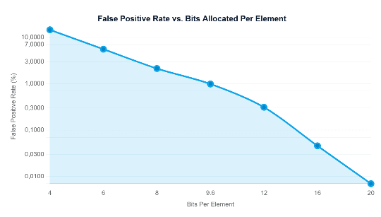
A widely cited rule of thumb confirms this curve in practice: a bloom filter requires fewer than 10 bits per element to achieve a 1% false positive rate, specifically around 9.6 bits per element, regardless of how large the elements themselves are. That last part is the real magic. Whether you are storing 8-byte keys or 200-byte URLs, the filter’s size depends only on how many items you store and how much error you are willing to tolerate, never on the size of the items.
Why Bloom Filters Are Everywhere
Inside Databases
Log-structured storage engines are the textbook use case. In systems built around the Log-Structured Merge tree architecture, writes land first in an in-memory memtable and are periodically flushed to disk as an immutable SSTable, and over time many SSTables accumulate per table. Without a shortcut, a single read could mean checking every one of those files. In Apache Cassandra, each SSTable has its own Bloom filter, a fixed-size bit array associated with that file. When a read request arrives, the filter is consulted first to check whether the requested partition key might exist in that SSTable, and if the filter returns a negative result, the request is rejected immediately without ever touching the disk. Cassandra even exposes this trade-off as a tunable operator setting. The bloom_filter_fp_chance parameter can be adjusted per table between 0 and 1, and typical values sit between 0.01 and 0.1, letting operators trade RAM for disk I/O depending on their hardware and workload.
Content Delivery Networks and Edge Caches
CDNs face a related problem at massive scale: deciding whether a requested object is cached at a given edge node before wasting a round trip. Rather than maintaining a full index of every cached object across every location, many caching layers use compact probabilistic summaries to quickly rule out misses, which keeps lookup latency low even as the catalog of cached content grows into the billions of entries.
Browsers and Security Checks
Bloom filters also found early fame in browser security. Google Chrome historically used a Bloom filter loaded with hashed malicious URLs so that any address typed into the browser was first checked locally, and only a hit against that local filter triggered a full server-side check. This meant the vast majority of safe browsing checks never required a network round trip at all, saving both time for the user and load on Google’s servers.
Bloom Filters vs the Alternatives
Bloom filters are not the only probabilistic membership structure, and it helps to see how they stack up against the exact alternative and against a close cousin designed to fix one specific limitation.
| Structure | Memory Use | False Positives | Supports Deletion | Best Fit |
|---|---|---|---|---|
| Hash Set | High, grows with element size | None | Yes | Small to medium datasets needing exact answers |
| Bloom Filter | Very low, fixed by count and target error rate | Tunable, small and known | No (standard form) | Large-scale existence checks before a costly lookup |
| Cuckoo Filter | Low, slightly higher than Bloom at same error rate | Tunable, small and known | Yes | Cases needing deletion support alongside compactness |
How Much Memory Do You Actually Save?
Numbers make the trade-off easier to feel. Picture a system that needs to track 10 million distinct keys. Storing them in a typical hash set means paying for object headers, hash buckets, internal pointers, and the string data itself, a cost that realistically lands somewhere around 100 bytes per entry once all that overhead is counted. A Bloom filter sized for a 1% error rate needs only its 9.6 bits per element, and one tuned for a stricter 0.1% error rate needs about 14.4 bits per element.
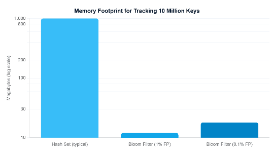
The gap is not subtle. A structure that would otherwise cost close to a gigabyte shrinks down to somewhere between 12 and 18 megabytes, all while giving up nothing more than a small, known, and controllable chance of an occasional unnecessary lookup.
| Target False Positive Rate | Bits Needed Per Element | Approx. Size for 10M Keys |
|---|---|---|
| 10% | ~4.8 bits | ~6 MB |
| 1% | ~9.6 bits | ~12 MB |
| 0.1% | ~14.4 bits | ~18 MB |
Quick Checklist: Is a Bloom Filter the Right Tool?
- You need a fast existence check before a more expensive operation, such as a disk read or network call.
- An occasional unnecessary check is acceptable, but a missed real match is not.
- The dataset is large enough that exact storage would be memory-prohibitive.
- You do not need to remove items later, unless you are using a variant like a Cuckoo filter or a Counting Bloom filter.
- You can tolerate rebuilding the filter when the underlying dataset changes significantly.
What We Learned
Bloom filters are a reminder that certainty is not always worth its price tag. By trading a small, mathematically predictable false positive rate for a dramatic drop in memory use, they let databases like Cassandra skip needless disk reads, let browsers filter dangerous sites locally, and let caches answer existence questions almost instantly at massive scale. The underlying idea is simple: know exactly when something is definitely absent, and be comfortable with an occasional, cheap double-check when it might be present. That single compromise is what makes Bloom filters one of the most quietly essential structures in modern infrastructure.