
Why the CAP theorem is frequently misunderstood, and how the PACELC model gives teams a more honest framework for database trade-offs.
Ask ten engineers to explain the CAP theorem, and you’ll likely get ten slightly different answers, several of them wrong in the same way. CAP has become one of those ideas that gets repeated in interviews and design docs far more often than it gets actually read from the source. That’s a shame, because the real insight buried underneath the buzzword is useful. It’s just incomplete. This is where PACELC steps in, quietly filling the gap that CAP leaves wide open.
What CAP Actually Says (and What It Doesn’t)
Eric Brewer’s original conjecture, later formalized by Seth Gilbert and Nancy Lynch in their 2002 proof, states that a distributed system cannot simultaneously guarantee Consistency, Availability, and Partition tolerance. The catch that most summaries skip is the condition under which this trade-off applies: only during a network partition. If the network is behaving, none of this forces a choice at all.
That single condition changes everything about how the theorem should be used. CAP is not a permanent personality trait of a database. It’s a description of what happens in one specific, hopefully rare, failure scenario.
The Most Common Misreading of CAP
The phrase “pick two out of three” is the most repeated and least accurate summary of CAP. Partition tolerance isn’t really optional for any system that runs across more than one machine — networks partition whether you planned for it or not. So in practice, every distributed database has already picked P, and the real decision is between C and A, and only during that partition window.
This leaves a much bigger question completely unanswered: what does the system do the other 99.9% of the time, when there is no partition at all? That’s precisely the question CAP was never designed to address, and it’s exactly what sends teams down the wrong path when comparing databases based on CAP labels alone.
Enter PACELC: The Missing Half of the Conversation
Daniel Abadi proposed PACELC in 2010, extending CAP with a second trade-off that applies during normal operation. Read as a single sentence, it says: if there is a Partition (P), choose between Availability (A) and Consistency (C); Else (E), choose between Latency (L) and Consistency (C).
| Condition | Trade-off | What it means in practice |
|---|---|---|
| During a partition (P) | A vs C | Serve possibly stale data, or refuse to serve at all |
| Normal operation (E) | L vs C | Respond fast with a local read, or wait for cross-node agreement |
The second half is the part most conversations about distributed databases quietly skip, even though it’s the trade-off engineers live with every single day, since partitions are the exception and normal operation is the rule.
How Real Databases Map onto PACELC
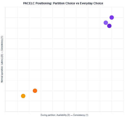
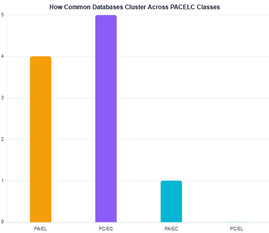
Classifying a system with a four-letter PACELC code turns out to be far more informative than a CAP label alone, because it captures both the rare-event behavior and the everyday behavior in one description.
| System | PACELC class | Everyday behavior |
|---|---|---|
| Amazon DynamoDB | PA/EL | Favors availability and low latency; consistency is tunable |
| Apache Cassandra | PA/EL (tunable) | Latency-optimized by default, consistency adjustable per query |
| MongoDB (default settings) | PC/EC | Favors consistency over both raw availability and lowest latency |
| Google Cloud Spanner | PC/EC | Strong consistency via synchronized clocks, at a latency cost |
| CockroachDB | PC/EC | Consensus-based writes prioritize consistency by design |
Why This Matters for Everyday Engineering Decisions
When a team picks a database based purely on its CAP classification, they’re really only planning for the failure case. PACELC forces a more honest question: what latency and consistency trade-off are we willing to accept on a completely healthy Tuesday afternoon? For a shopping cart, slightly stale reads are usually harmless, so leaning toward EL makes sense. For a ledger recording financial transactions, the opposite is true, and EC is worth the added latency.
This is also why comparing two “AP” databases side by side can still lead to very different production outcomes. Two systems can make the same choice during a partition and completely different choices the rest of the time, and it’s that second choice that shapes user-facing latency every single day.
A Practical Way to Apply PACELC
Before choosing a database for a new service, ask:
- What actually happens to our users if this system briefly serves stale data during a rare network partition?
- On a normal day, is a slower, strongly consistent read acceptable, or does the user experience depend on low latency?
- Are these two answers actually the same trade-off, or do they pull in different directions?
- Does the database expose tunable consistency, or is the PACELC class fixed by design?
- Have we tested behavior under partition, not just under normal load, before trusting the vendor’s label?
Tunable systems like Cassandra add a layer worth remembering: the PACELC class isn’t always a single fixed answer, it can shift per query depending on the consistency level requested, which means the trade-off decision moves from the database vendor to the engineer writing the query.
What We Learned
The CAP theorem answers a narrower question than most engineers assume: it only describes what a system does during a network partition, and even then it reduces to a choice between availability and consistency since partition tolerance isn’t really optional. PACELC completes the picture by adding the trade-off that governs everyday operation — latency versus consistency — which is the one most services actually live with day to day. Classifying a database by its full four-letter PACELC code, rather than its CAP label alone, gives a far more honest basis for choosing the right system for a given workload, and for understanding why two “AP” databases can still feel completely different in production.