Modern data engineering rarely lives on a single machine. As datasets grow from gigabytes into terabytes — and sometimes into petabytes — teams need orchestration tools that can schedule, retry, and monitor dozens of interdependent pipeline steps without requiring engineers to babysit every run. That is precisely the problem that Apache Airflow solves, and when paired with Google BigQuery on GCP, the combination becomes one of the most capable stacks available for production-grade data processing.
In this article we walk through the full picture: what these two tools are, how they connect, how to build a practical pipeline that moves data from Google Cloud Storage (GCS) into BigQuery, and the patterns that keep things fast, cost-efficient, and maintainable as the pipeline grows.
The Two Tools and Why They Belong Together
Before writing a single line of Python, it helps to understand what each service brings to the table — and why they complement each other so naturally.
Apache Airflow is an open-source workflow orchestration platform that lets you define pipelines as Directed Acyclic Graphs (DAGs). A DAG is simply a Python file that describes tasks and the dependencies between them. Airflow schedules those tasks, tracks their state, handles retries on failure, and gives you a web UI to monitor everything in real time. According to VentureBeat, Airflow has become the de facto standard for data engineering and has been adopted by Fortune 500 companies worldwide.
Google BigQuery, on the other hand, is a fully-managed, serverless data warehouse capable of analysing petabytes of data using familiar SQL. It decouples storage from compute — meaning you pay for what you scan, not for idle servers. On-demand pricing currently sits at around $6.25 per terabyte of data processed, with the first 1 TB free each month.
The key insight is that Airflow and BigQuery operate at different layers. Airflow orchestrates when and in what order things run; BigQuery does the heavy computational lifting. Together, they give you scheduling intelligence and near-unlimited analytical scale in a single, coherent pipeline.
Setting Up Cloud Composer 3
On GCP, the managed way to run Airflow is Cloud Composer. With Cloud Composer 3 — the current generation — Google handles Airflow scheduler upgrades, worker autoscaling, and the underlying GKE cluster entirely for you. All you need to manage are your DAG files.
Creating an environment is straightforward from the GCP Console. Navigate to Cloud Composer, click Create environment, choose Composer 3, and select an Airflow version (2.9.x or 2.10.x are current). Once the environment is up — which typically takes around 15 to 20 minutes — you configure the BigQuery connection inside Airflow’s Admin panel.
From there, deploying DAGs is simply a matter of uploading Python files to the environment’s GCS DAGs bucket. Cloud Composer picks them up automatically within a minute or two. No restart required.
Important migration note: All Cloud Composer 1 environments and Composer 2 versions 2.0.x will reach end of life on September 15, 2026. If you are still on these versions, plan your migration to Cloud Composer 3 now.
Installing the Google Provider Package
Airflow’s BigQuery operators live in the apache-airflow-providers-google package. In a Cloud Composer environment this comes pre-installed, but if you are running self-hosted Airflow you will need to add it explicitly. The package gives you a full suite of operators for interacting with BigQuery, GCS, Dataflow, and most other GCP services.
The key operators you will reach for most often in a BigQuery pipeline are listed below.
| Operator | What it does | Typical use |
|---|---|---|
GCSToBigQueryOperator | Loads files from GCS directly into a BigQuery table | Daily / hourly ingestion from a data lake |
BigQueryInsertJobOperator | Executes any BigQuery job: query, load, extract, or copy | Transformations, aggregations, ELT logic |
BigQueryCheckOperator | Runs a query and fails the task if the result is falsy | Data quality gates |
BigQueryTableExistenceSensor | Pauses the DAG until a specified table exists | Cross-DAG dependency waiting |
BigQueryCreateEmptyDatasetOperator | Creates a dataset if it does not already exist | First-run bootstrapping |
Building a Production-Ready DAG
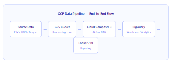
Let us now look at a realistic, end-to-end DAG. The pipeline below does three things: it loads a daily Parquet file from GCS into a staging table, runs a transformation query that writes results to a partitioned production table, and then runs a data quality check. This ELT pattern — Extract, Load, then Transform inside BigQuery — is the most common approach in modern GCP data stacks because it moves heavy computation to where it is cheapest and most scalable.
# gcs_to_bq_pipeline.py
from datetime import datetime, timedelta
from airflow.sdk import DAG
from airflow.providers.google.cloud.operators.bigquery import (
    BigQueryInsertJobOperator,
    BigQueryCheckOperator,
)
from airflow.providers.google.cloud.transfers.gcs_to_bigquery import GCSToBigQueryOperator

PROJECT_ID  = "my-gcp-project"
DATASET     = "analytics"
STAGING_TBL = "events_staging"
PROD_TBL    = "daily_events"
GCS_BUCKET  = "my-data-lake-bucket"

default_args = {
    "owner":       "data-engineering",
    "retries":     2,
    "retry_delay": timedelta(minutes=5),
}

with DAG(
    dag_id="gcs_to_bigquery_daily",
    default_args=default_args,
    schedule="0 6 * * *",          # run at 06:00 UTC every day
    start_date=datetime(2025, 1, 1),
    catchup=False,
    tags=["bigquery", "etl", "gcs"],
) as dag:

       # ── Step 1: load raw Parquet from GCS into a staging table ──────────────
    load_to_staging = GCSToBigQueryOperator(
        task_id="load_raw_to_staging",
        bucket=GCS_BUCKET,
        source_objects=["events/{{ ds }}/data.parquet"],
        destination_project_dataset_table=(
            f"{PROJECT_ID}.{DATASET}.{STAGING_TBL}"
        ),
        source_format="PARQUET",
        write_disposition="WRITE_TRUNCATE",  # replace staging each run
        autodetect=True,
        gcp_conn_id="google_cloud_default",
    )

     # ── Step 2: transform and write to partitioned production table ──────────
    transform_and_load = BigQueryInsertJobOperator(
        task_id="transform_to_prod",
        configuration={
            "query": {
                "query": """
                    INSERT INTO `my-gcp-project.analytics.daily_events`
                    SELECT
                        DATE(event_timestamp)   AS event_date,
                        event_type,
                        user_id,
                        COUNT(*)                AS event_count
                    FROM  `my-gcp-project.analytics.events_staging`
                    WHERE DATE(event_timestamp) = '{{ ds }}'
                    GROUP BY event_date, event_type, user_id
                """,
                "useLegacySql": False,
            }
        },
        gcp_conn_id="google_cloud_default",
    )

     # ── Step 3: data quality gate — fail if no rows were inserted ───────────
    quality_check = BigQueryCheckOperator(
        task_id="row_count_check",
        sql="""
            SELECT COUNT(*) > 0
            FROM `my-gcp-project.analytics.daily_events`
            WHERE event_date = '{{ ds }}'
        """,
        use_legacy_sql=False,
        gcp_conn_id="google_cloud_default",
    )

     # ── Task order ───────────────────────────────────────────────────────────
    load_to_staging >> transform_and_load >> quality_check
A few things are worth calling out in this DAG. First, the {{ ds }} template variable is Airflow’s built-in date shorthand — it resolves to the execution date of each run in YYYY-MM-DD format. This means the pipeline is naturally idempotent: re-running a past date always targets the same partition of data. Second, catchup=False prevents Airflow from backfilling all missed runs if the DAG is paused and then re-enabled, which is almost always the right default in production. Third, the three-step linear dependency chain (>> operator) ensures quality checks never run against a table that failed to load.
Template tip: Airflow’s Jinja templating also exposes {{ ds_nodash }} (e.g. 20250614) and {{ prev_ds }} (yesterday). These are invaluable for building partition-aware table suffixes and date-range filters directly inside your SQL.
Partitioning and Clustering — The Single Biggest Performance Lever
One of the most important BigQuery best practices is to never let a query scan more data than it needs. Even with on-demand pricing at $6.25 per terabyte, a handful of full-table scans per day on a 10 TB table can quietly compound into a serious bill. Partitioning and clustering solve this at the storage layer, before a single slot of compute is consumed.
Partitioning splits a table into segments by a column — most commonly a DATE or TIMESTAMP field. When a query filters on that column, BigQuery skips partitions that do not match entirely. Clustering goes further by sorting the data within each partition by one or more additional columns, allowing BigQuery to skip individual blocks rather than entire partitions.
When creating a production table that will be loaded by your DAG, define both at the schema level with a simple DDL statement in a BigQueryInsertJobOperator:
# Create the partitioned + clustered destination table (run once, or idempotently)
create_prod_table = BigQueryInsertJobOperator(
    task_id="create_prod_table",
    configuration={
        "query": {
            "query": """
                CREATE TABLE IF NOT EXISTS
                    `my-gcp-project.analytics.daily_events`
                (
                    event_date   DATE,
                    event_type   STRING,
                    user_id      STRING,
                    event_count  INT64
                )
                PARTITION BY event_date
                CLUSTER BY   event_type, user_id
            """,
            "useLegacySql": False,
        }
    },
    gcp_conn_id="google_cloud_default",
)
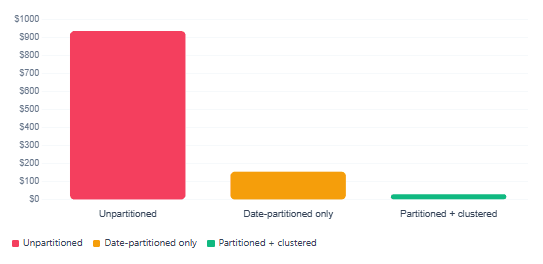
With this in place, a query filtering on event_date = '2025-06-14' AND event_type = 'purchase' will skip everything outside that date partition and then skip blocks within the partition that do not contain purchase events. In practice, this routinely reduces scanned data by 90% or more on large tables.
Query scan cost — unpartitioned vs. partitioned + clustered table
Connecting the GCS and BigQuery Authentication
Everything in the DAG above routes authentication through the google_cloud_default connection ID. In Cloud Composer 3, this connection is pre-configured with the environment’s service account, so no extra setup is required for BigQuery access within the same GCP project. For cross-project access — or when running self-hosted Airflow — you need to configure the connection manually.
To do that, go to Airflow UI → Admin → Connections, create a new connection with:
| Field | Value |
|---|---|
| Conn ID | google_cloud_default |
| Conn Type | Google Cloud |
| Keyfile JSON / Path | Path to service account JSON key, or leave blank for Workload Identity |
| Project ID | Your GCP project ID |
| Scopes | https://www.googleapis.com/auth/cloud-platform |
Security note: Avoid storing JSON service account keys on disk in production environments. Instead, use Workload Identity Federation, which binds the Airflow worker’s Kubernetes service account to a GCP service account without any key file. Cloud Composer 3 supports this natively.
Error Handling and Retries
Production data pipelines fail. Network blips happen, BigQuery slots are occasionally exhausted, and source files sometimes arrive late. Airflow’s retry mechanism is, therefore, one of its most important features — and it is straightforward to configure at both the DAG level and the individual task level.
The default_args dictionary in your DAG sets baseline retry behaviour for all tasks. You can override it on any specific task that needs different treatment. For tasks that call external APIs or load large files, a small exponential backoff is often worth adding:
from airflow.utils.trigger_rule import TriggerRule

# A cleanup task that runs even if upstream tasks fail
cleanup = BigQueryInsertJobOperator(
    task_id="truncate_staging",
    configuration={
        "query": {
            "query": "TRUNCATE TABLE `my-gcp-project.analytics.events_staging`",
            "useLegacySql": False,
        }
    },
    trigger_rule=TriggerRule.ALL_DONE,  # runs regardless of upstream success/failure
    retries=1,
    retry_delay=timedelta(minutes=2),
    gcp_conn_id="google_cloud_default",
)

# Add cleanup to the end of the chain
quality_check >> cleanup
The TriggerRule.ALL_DONE setting ensures that the staging table is always cleaned up at the end of a run, even when an earlier task fails. This prevents stale data from leaking into the next day’s load — a subtle but important production concern that is easy to overlook when building a pipeline for the first time.
Monitoring Your Pipeline
Once a DAG is running in production, you need visibility into its health. Airflow’s built-in web UI shows task durations, success and failure history, and a Gantt chart view per DAG run. For deeper observability, Cloud Composer 3 forwards all Airflow logs to Cloud Logging automatically, and you can create metric-based alerts in Cloud Monitoring — for example, an alert when a DAG run exceeds its expected duration or when task failure rates spike.
On the BigQuery side, the INFORMATION_SCHEMA.JOBS view is an invaluable tool for tracking query costs and slot consumption per pipeline run. The following query surfaces the top cost-generating jobs in the past 24 hours:
SELECT
    job_id,
    query,
    total_bytes_processed / POW(10, 12) AS tb_processed,
    ROUND(total_bytes_processed / POW(10, 12) * 6.25, 4) AS estimated_cost_usd,
    creation_time
FROM `region-us`.INFORMATION_SCHEMA.JOBS
WHERE
    creation_time >= TIMESTAMP_SUB(CURRENT_TIMESTAMP(), INTERVAL 24 HOUR)
    AND job_type = 'QUERY'
    AND state    = 'DONE'
ORDER BY total_bytes_processed DESC
LIMIT 20;
Running this regularly — or scheduling it as its own Airflow task that writes results to a monitoring dataset — gives you ongoing cost visibility without needing to open the GCP billing console every time.
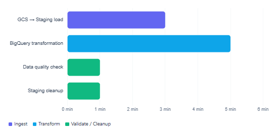
Typical Airflow + BigQuery pipeline task duration breakdown
Key Best Practices at a Glance
Before wrapping up, it is worth consolidating the practical recommendations that cut across everything we have discussed. These are the habits that separate a pipeline that merely works from one that holds up reliably at scale.
| Practice | Why it matters |
|---|---|
Use catchup=False in all production DAGs | Prevents unexpected backfill runs after a DAG is re-enabled |
Set WRITE_TRUNCATE on staging, WRITE_APPEND on production | Keeps staging tables clean while accumulating history in production |
| Partition by date, cluster by filter columns | Cuts query costs by 80–95% on large tables |
Use {{ ds }} and {{ ds_nodash }} in SQL | Makes every DAG run idempotent and safely re-runnable |
Add a BigQueryCheckOperator after each load | Catches empty or incomplete loads before downstream steps consume bad data |
| Store secrets in Secret Manager, not in connection keyfiles | Reduces credential exposure; Cloud Composer 3 integrates natively |
| Use Workload Identity instead of JSON keys | Eliminates key rotation overhead and reduces attack surface |
Monitor with INFORMATION_SCHEMA.JOBS | Gives per-query cost visibility without leaving BigQuery |
What We Learned
We covered how Apache Airflow and BigQuery each occupy a distinct layer of a GCP data pipeline — Airflow handles orchestration and scheduling through DAGs while BigQuery provides the serverless analytical compute. We set up a Cloud Composer 3 environment, walked through the key BigQuery operators (GCSToBigQueryOperator, BigQueryInsertJobOperator, and BigQueryCheckOperator), and built a complete, production-ready ELT DAG that loads Parquet files from GCS into a staging table, transforms them into a partitioned production table, and validates the result.
We then explored why partitioning and clustering are the single most impactful cost-control levers in BigQuery, how authentication works through Workload Identity in Cloud Composer 3, how to handle failures and cleanup with Airflow’s trigger rules, and how to monitor both DAG health and BigQuery query costs through Airflow’s UI, Cloud Monitoring, and INFORMATION_SCHEMA.JOBS.
