Shannon’s 1948 paper defined the theoretical limits of data compression — and quietly seeded ideas that now live inside your compression algorithms, ML models, database query planners, and security tools. Here is what the theory actually says, with no hand-waving.
You have probably seen the word “entropy” used loosely — as a metaphor for code complexity, system disorder, or the general drift of software toward chaos. That is not what Claude Shannon meant by it. When Shannon published A Mathematical Theory of Communication in the Bell System Technical Journal in 1948, he gave entropy a precise, computable, and deeply useful definition that has nothing to do with disorder in the poetic sense.
Shannon entropy measures how much uncertainty exists in a probability distribution. More practically: it tells you the minimum average number of bits required to encode the outcomes of a random process. That definition turns out to be the theoretical foundation for ZIP files, the split logic in a decision tree, the strength metric on a password field, and the way a database optimizer decides whether a full table scan is cheaper than an index lookup. Understanding it properly — not as a metaphor — makes each of those systems legible in a new way.
1. What entropy actually measures
Start with the intuition. If someone tells you something you already knew with certainty, they have communicated zero information. If they tell you the outcome of a fair coin flip — something with maximum unpredictability — they have communicated as much information as a single binary choice can carry. Shannon’s key insight, as Quanta Magazine describes it, is that information is maximised when surprise is maximised.
The formula that formalises this is elegantly compact. For a discrete random variable X with possible outcomes x₁, x₂, … xₙ and associated probabilities p₁, p₂, … pₙ:
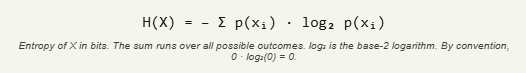
Each term − log₂ p(xᵢ) is the “surprise” of seeing outcome xᵢ — the number of bits you would need to encode the information that this specific outcome occurred. Multiply each surprise by how likely that outcome is, sum them up, and you get the expected surprise across the whole distribution. That expected value is Shannon entropy.
Three concrete examples that build intuition
Consider these distributions and their entropies. A fair coin has two outcomes, each with probability 0.5. A loaded coin always lands heads. An eight-sided die has eight equally probable faces. Notice how the entropy tracks your intuition about uncertainty perfectly:
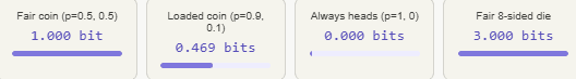
The loaded coin at 0.469 bits is particularly instructive. You still do not know for certain what it will show — but you are pretty confident it is heads. Your uncertainty is less than half of what it would be with a fair coin, and the entropy reflects that precisely. A uniform distribution — where every outcome is equally likely — always achieves the maximum possible entropy for a given number of outcomes. That maximum is log₂(n) bits, where n is the number of outcomes.
The source coding theorem (Shannon’s first major result): No lossless compression scheme can compress a sequence of symbols to fewer bits on average than H(X) bits per symbol. This is not a limitation of today’s algorithms — it is a mathematical impossibility. ZIP files, LZ77, Huffman coding — none of them can do better, on average, than the entropy of the source.
2. Mutual information: what one variable tells you about another
Entropy describes a single variable in isolation. Mutual information extends the idea to the relationship between two variables. Specifically, the mutual information I(X; Y) between X and Y measures how much knowing X reduces your uncertainty about Y — or equivalently, how much knowing Y reduces your uncertainty about X. The definition is symmetric: I(X; Y) = I(Y; X).
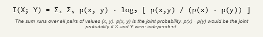
This formula has a clean interpretation. If X and Y are completely independent, then p(x, y) = p(x) · p(y) for every pair, and every log term evaluates to log₂(1) = 0, so I(X; Y) = 0 — knowing X tells you nothing about Y. If, on the other hand, Y is a deterministic function of X, then I(X; Y) = H(Y): knowing X eliminates all uncertainty about Y.
There is also a clean relationship between mutual information and entropy that is worth keeping in mind:

Equally useful is the conditional entropy formulation:

Shannon entropy of a binary variable as a function of probability p — the characteristic concave curve peaking at p = 0.5

3. Application 1: Data compression and Huffman coding
Shannon’s source coding theorem says that the entropy of a source is the fundamental lower bound on compression. However, it also tells you something practically useful: the further a real source’s entropy is from its naive encoding length, the more room there is to compress it.
Consider English text. The 26 lowercase letters each occur with very different frequencies — ‘e’ is far more common than ‘z’. A naive fixed-width encoding would use log₂(26) ≈ 4.7 bits per character regardless. However, Shannon estimated the actual entropy of English text at roughly 1.0–1.5 bits per character by measuring how well humans could predict the next letter in a sentence — because structure and predictability reduce entropy. The gap between 4.7 bits and ~1.1 bits is why a compressed text file can be a fraction of the original size.
Huffman coding (the basis of many real compression formats) directly implements this insight. It assigns shorter bit codes to more probable symbols and longer codes to rarer ones. A character with probability 0.5 gets a 1-bit code; one with probability 0.25 gets a 2-bit code. The average code length converges to the Shannon entropy of the source. Huffman codes are provably optimal for symbol-by-symbol coding — they cannot, on average, do better than H(X) bits per symbol, and they achieve it.
This is also why compression ratios are data-dependent in a precise, measurable way. A file of random bytes has an entropy close to 8 bits per byte (the maximum), and no compression algorithm will make it meaningfully smaller — it is already at its information-theoretic limit. A sparse log file or natural-language document, by contrast, has much lower entropy and compresses well. Trying to compress an already-compressed file (like a JPEG inside a ZIP) rarely helps — and sometimes makes it slightly larger — for exactly this reason.
4. Application 2: Decision trees and feature selection in machine learning
Shannon entropy is embedded directly into the logic of decision tree algorithms. When a decision tree algorithm like ID3 or C4.5 decides which feature to split on at a given node, it measures information gain — which is simply mutual information between the feature and the target label.
Information gain, concretely
Suppose you have a dataset D with a binary label (pass/fail). The entropy of D is H(D) — computed from the proportion of passing and failing examples. Now you consider splitting D by some feature A (say, “study hours > 5”). You get two subsets Dᵥ, one for each value of A. The information gain is:

ID3 greedily picks the feature with the highest information gain at each step. The intuition is clean: you want to pick the question that, on average, tells you the most about the answer. That is precisely what mutual information measures.
A known limitation: Raw information gain is biased toward features with many distinct values (like a unique ID column, which would give a perfect split but is useless for generalisation). C4.5 addresses this with gain ratio, which normalises IG by the entropy of the feature itself. The deeper lesson is that entropy-based metrics are powerful but must be applied with care — the formula does not automatically know what is meaningful.
Mutual information for feature selection
Beyond decision trees, mutual information is used directly for feature selection in any ML pipeline. Given a feature X and target Y, I(X; Y) measures how much knowing X reduces uncertainty about Y — without making any assumption about whether the relationship is linear. This is a significant advantage over correlation coefficients, which only detect linear dependencies. A feature with high I(X; Y) is informative regardless of the shape of the relationship. In scikit-learn, mutual_info_classif computes this for each feature against the target, making it a practical, model-agnostic relevance filter before training.
Cross-entropy: the loss function connection
One more ML connection worth naming: the cross-entropy loss used in neural network training is directly information-theoretic. For a true distribution p and a model’s predicted distribution q, the cross-entropy is H(p, q) = −Σ p(x) log₂ q(x). Minimising cross-entropy loss is equivalent to making your model’s predicted distribution as close as possible to the true distribution. The minimum achievable cross-entropy is the entropy of the true distribution H(p) itself — another manifestation of Shannon’s source coding theorem.
How information gain works in a decision tree: entropy before and after a split (illustrative example, binary classification, 10-sample dataset)

5. Application 3: Database query optimisation and cardinality estimation
Every time a database optimizer decides between a sequential scan and an index lookup, or between a hash join and a nested loop join, it needs to estimate how many rows a given condition will return. This is the cardinality estimation problem, and it is fundamentally a problem of reasoning about distributions — which brings in entropy, even if the word never appears in a SQL manual.
The core mechanism in databases like PostgreSQL is the histogram. For each column, the optimizer maintains a summary of the value distribution. When you write WHERE age > 30, the planner consults this histogram to estimate what fraction of rows satisfy the condition — the selectivity. That estimate drives the entire query plan.
| Column characteristic | Effective entropy | Optimizer implication |
|---|---|---|
| Boolean flag (95% true / 5% false) | Low (~0.29 bits) | High selectivity; index on rare value (false) is very useful |
| Country code (50 countries, roughly uniform) | Medium (~5.6 bits) | Index moderately useful; depends on query filter |
| UUID primary key (fully random) | Maximum (~32+ bits) | Equality lookup: index essential. Range scan: almost never useful |
| Created_at timestamp (clustered writes) | Medium-high but skewed | Histogram buckets capture the skew; uniform assumption would badly mis-estimate recent data |
Intuitively: a column with low entropy has a very predictable, concentrated distribution. A filter condition on such a column is either very selective (touching the rare values) or very unselective (touching the common values). The optimizer needs the histogram to tell which case applies. A high-entropy, nearly-uniform column is predictable in a different way — uniform selectivity — and the optimizer’s uniform assumption is actually reasonable for it.
The deeper connection is that optimal histogram construction — deciding how wide to make each bucket — is an entropy-maximisation problem. Buckets should be positioned so that the assumed-uniform distribution within each bucket is as accurate as possible, which means distributing the “information content” of the column evenly across buckets. The academic literature formalises this: one influential paper by Kaushik, Re, and Suciu proposes using maximum-entropy distributions as the principled basis for all database cardinality estimation, ensuring that every statistical assertion a planner makes is as non-committal as possible given the available evidence.
6. Application 4: Security — password strength and anomaly detection
Password entropy
When you see a password strength bar on a registration form, the underlying concept — whether the implementation acknowledges it or not — is Shannon entropy. A password drawn uniformly at random from an alphabet of size N with length L has entropy:

This is exactly what Wikipedia’s treatment of password strength and NIST guidelines formalise: a password with 42 bits of entropy requires 2⁴² attempts to exhaust all possibilities; adding one bit doubles that count. The critical nuance — which caused NIST to revise their SP 800-63 guidance in 2017 — is that the formula above applies to truly random passwords. Human-generated passwords have far lower entropy than their character-pool would suggest, because people are predictably bad at being random. Measuring the actual entropy of human password distributions requires studying real-world password leaks, and those studies consistently find that people cluster around familiar patterns.
A subtlety engineers often miss: High entropy and strong password are not synonyms when humans are involved. A password like “Tr0ub4dor&3” that hits all the character-set categories has a character-pool entropy of ~52 bits, but because its structure is predictable (word + substitutions + number + symbol), its real-world entropy is much lower. This is precisely why NIST’s 2017 revision moved away from complexity rules toward length-and-uniqueness requirements.
Entropy in anomaly detection
Network security and log monitoring systems use entropy to detect anomalies. The key idea is that legitimate traffic or well-behaved logs tend to have a characteristic entropy profile. A DNS server under normal operation shows moderate entropy in the domain names it resolves — real domains have structure and repetition. Domain generation algorithms (DGAs) used by malware to find command-and-control servers generate domain names that look random and therefore have much higher per-character entropy. Measuring the Shannon entropy of observed hostnames is therefore a practical first-pass signal for DGA-based malware detection. Similarly, data exfiltration through DNS tunnelling (encoding stolen data in DNS queries) produces unusually high-entropy query strings that stand out from the baseline.
7. Where these concepts live in systems you use daily

8. What we have learned
Shannon entropy — H(X) = −Σ p(xᵢ) · log₂ p(xᵢ) — is a single, elegant quantity that measures the average uncertainty in a probability distribution. It tells you the minimum average bits needed to encode a source (the source coding theorem), and its maximum value is log₂(n) bits for n equally probable outcomes. Mutual information I(X; Y) extends this to measure the statistical dependence between two variables — how much knowing one reduces uncertainty about the other — capturing linear and non-linear relationships alike.
In compression, entropy is the hard lower bound that no lossless algorithm can break. In decision trees and feature selection, information gain is mutual information between a feature and the label, and it drives the greedy split logic in ID3, C4.5, and XGBoost. In databases, histogram-based cardinality estimation is implicitly reasoning about column entropy distributions, and the principled form of this reasoning is maximum-entropy modelling. In security, password entropy quantifies brute-force resistance, and entropy measurement on network traffic or DNS queries is a practical anomaly detection signal.
The unifying thread is this: whenever you are trying to ask “how much information does variable X carry about Y?”, or “what is the theoretical limit on how compactly I can represent this data?”, or “how predictable is this distribution?”, you are asking a Shannon entropy question. Having the right vocabulary and the right formula makes each of these problems considerably more tractable — and considerably less mysterious.
