The invisible infrastructure powering semantic search, RAG, and recommendations — and how to pick the right one without regretting it later.
Every time a chatbot pulls up a document that actually matches your question, or a music app recommends a song that somehow fits your mood, a vector database did the heavy lifting. These systems have gone from niche ML infrastructure to the backbone of nearly every serious AI product built in the last two years — and the market is catching up fast.
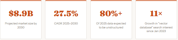
The vector database market is expected to be worth $2.65 billion in 2025 and reach $8.95 billion by 2030, growing at a CAGR of 27.5%. That’s not hype — it’s a reflection of how deeply these systems are embedded in the AI application stack. If you’re building anything AI-native right now, you need to understand this layer.
1. What a Vector Database Actually Does
Traditional databases store data in rows and columns and answer questions like “find all users where country = ‘Greece’.” That model breaks down the moment your question is semantic — “find content that is similar in meaning to this paragraph” or “find products that look like this image.” For that, you need vectors.
A vector is a list of numbers — typically hundreds or thousands of them — that encodes the meaning or content of a piece of data. A machine learning embedding model converts text, images, audio, or video into these vectors. Once you have vectors, you can measure how similar two pieces of content are by calculating the distance between them in that high-dimensional space. Vectors that are close together are similar in meaning. A vector database’s job is to do this at scale and at speed.
Searching by meaning, not by keyword — that’s the fundamental shift vector databases unlock.
How the Search Works: HNSW
Almost every modern vector database uses an algorithm called HNSW — Hierarchical Navigable Small World — for approximate nearest neighbor (ANN) search. Think of it as a multi-layered graph: the top layer has a small number of broadly connected nodes, and each layer below gets denser and more specific. When you issue a query, the search starts at the top and navigates down, narrowing in on the best matches rapidly. This is why a properly indexed vector database can find the 10 most similar items among 50 million vectors in milliseconds — without checking every single one.
The three knobs that control HNSW behavior are m (connections per node — higher means better accuracy but more memory), ef_construct (quality of index build — higher is slower to build but more accurate), and hnsw_ef (search candidates at query time — trade latency for accuracy).
2. The Contenders in 2025–2026
The landscape has matured significantly. There are now six categories of players: purpose-built managed services, purpose-built self-hosted, PostgreSQL extensions, full-featured databases with vector bolt-ons, serverless newcomers, and legacy search engines with vector support. Here’s the honest map:
| Database | Type | Index | Hybrid Search | Best For | Pricing |
|---|---|---|---|---|---|
| Pinecone | Managed | Proprietary | Native | Fast time-to-prod, no infra ops | Usage-based, free tier |
| Weaviate | OSS / Cloud | HNSW + ACORN | Native | Hybrid search, multimodal | Free OSS, cloud pricing |
| Qdrant | OSS / Cloud | Filterable HNSW | Native | Filtered search, Rust performance | 1GB free forever, pay-as-you-go |
| Milvus | OSS / Cloud | HNSW, IVF, DiskANN | Native | Billion-scale, enterprise | Free OSS, Zilliz Cloud |
| pgvector + pgvectorscale | Extension | HNSW + DiskANN | Partial | Postgres teams, moderate scale | Free (infra cost only) |
| Chroma | OSS | HNSW | Yes | Prototyping, local dev | Free OSS |
| Turbopuffer | Serverless | Custom | Yes | Cost-sensitive, AI prod teams | ~$9 / 1M reads+writes |
QPS at 99% Recall — 50M Vectors (768 dimensions)
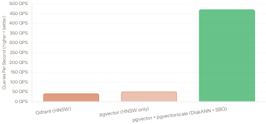
That chart deserves a double-take. In terms of throughput at 99% recall, Postgres with pgvector and pgvectorscale demonstrates significantly higher capacity on a single node, achieving 11.4x more throughput than Qdrant — 471.57 queries per second versus 41.47 QPS — on 50 million embeddings. This was a surprising result that challenged the assumption that purpose-built specialized databases would always outperform a general-purpose database with extensions. That said, index build times are faster in Qdrant, which matters if you’re doing frequent writes or near-real-time indexing. And Qdrant’s filterable HNSW gives it strong advantages in filtered search workloads, which the raw QPS number doesn’t capture.
3. Filtering: The Real Battlefield
Raw throughput benchmarks tell you one thing. But most production AI applications don’t just ask “find me the 10 nearest vectors” — they ask “find me the 10 nearest vectors where category = ‘electronics’ and price < 200.” That’s filtered vector search, and it’s where the databases diverge sharply.
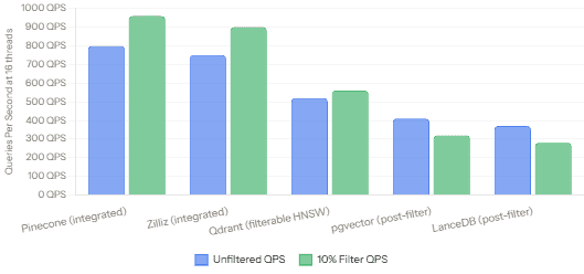
There are three approaches: post-filtering (run ANN first, filter afterward — fast but loses results when filters are tight), pre-filtering (filter down the dataset first, then run ANN over the subset — accurate but slow and memory-hungry), and integrated filtering (modifying the ANN algorithm itself to respect filters inline). Engines with in-algorithm filtering not only preserve recall — they actually get faster, more predictable searches when filters prune the workload.
Integrated Filtering — Who Does It Best
Qdrantuses a filterable HNSW with an adaptive query planner that picks between graph traversal and brute force based on selectivity.Weaviateuses ACORN — a two-hop graph expansion that keeps recall high under selective filters.Pineconemerges metadata and vector indexes in a single-stage search, which is why its latency can actually drop under tight filters.
Multi-Threaded QPS — Unfiltered vs 10% Filter (16 threads)
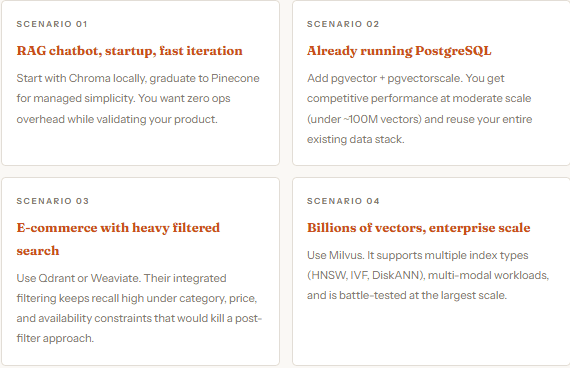
4. Real Use Cases, Matched to the Right Tool
Choosing a vector database isn’t just about benchmarks — it’s about fit. The same engine that powers Pinecone’s $130M-backed managed service is not necessarily the right tool for a solo developer prototyping a RAG chatbot. Here’s how to think about it:
5. RAG and Why Vector DBs Are Central to It
Retrieval-Augmented Generation (RAG) is the dominant pattern for building production AI applications right now. The idea is simple: instead of asking an LLM to answer from its training data alone, you first retrieve relevant context from your own documents using a vector search, then pass that context into the prompt. The model answers based on real, up-to-date information rather than guessing.
The vector database is the retrieval engine in this workflow. At query time, your user’s question gets embedded into a vector, the database finds the most semantically similar document chunks, and those chunks become the context window for the LLM. The quality of that retrieval step — how fast it is, how accurate, how well it handles filters like date or document type — directly determines the quality of the final answer.
In a RAG system, the quality of the LLM’s answer is bounded by the quality of the retrieval step. Your vector database is not a detail — it’s load-bearing.
Hybrid Search: The Right Default
Pure vector search misses exact matches. Pure keyword search misses semantic meaning. Hybrid search — combining BM25 keyword matching with HNSW vector similarity in a single query — gives you both. Weaviate, Qdrant, Turbopuffer, and Elasticsearch support hybrid search natively. Cloudflare Vectorize notably does not. For most RAG workloads, hybrid search meaningfully improves recall without adding significant latency. Enable it by default if your database supports it.
6. Getting Started: A Minimal Qdrant Setup
To make this concrete, here’s a complete, runnable example using Qdrant — one of the most popular open-source options. You can run Qdrant locally via Docker with zero configuration. The Python client is pip-installable.
# Step 1 — Run Qdrant locally (requires Docker)
docker run -p 6333:6333 qdrant/qdrant

# Step 2 — Install the Python client
pip install qdrant-client sentence-transformers
# Step 3 — Create a collection, index documents, and search
from qdrant_client import QdrantClient
from qdrant_client.models import Distance, VectorParams, PointStruct
from sentence_transformers import SentenceTransformer

# Connect to local Qdrant
client = QdrantClient(host="localhost", port=6333)
model = SentenceTransformer("all-MiniLM-L6-v2")  # 384-dim embeddings

# Create a collection
client.create_collection(
    collection_name="articles",
    vectors_config=VectorParams(size=384, distance=Distance.COSINE),
)

# Add some documents
docs = [
    "Vector databases power semantic search in AI apps.",
    "HNSW is the most common ANN algorithm in vector search.",
    "RAG combines retrieval with large language models.",
]
vectors = model.encode(docs).tolist()

client.upsert(
    collection_name="articles",
    points=[PointStruct(id=i, vector=v, payload={"text": d})
            for i, (v, d) in enumerate(zip(vectors, docs))],
)

# Search — find the most semantically similar doc
query_vector = model.encode("how does approximate nearest neighbor work?").tolist()
results = client.search(collection_name="articles", query_vector=query_vector, limit=1)

print(results[0].payload["text"])
# Output: "HNSW is the most common ANN algorithm in vector search."
This runs entirely on your laptop — no cloud account needed. The all-MiniLM-L6-v2 model is a fast, lightweight sentence transformer that produces 384-dimensional embeddings, well suited for RAG prototyping. Swap in a larger model like OpenAI's text-embedding-3-large (3072 dimensions) when you need higher accuracy at scale.
7. What to Watch: The Road Ahead
The vector database space is moving quickly. A few developments worth watching:
Traditional databases are catching up. SQL Server 2025, Oracle Autonomous, and MongoDB all added or significantly improved native vector support in 2024–2025. The fundamentals remain: you need a vector database that balances performance, scale, cost, and operational complexity for your specific use case. But the era where “vector database” meant a separate specialized system may be shorter than vendors expected.
Serverless is gaining ground. Turbopuffer has quietly become the choice of production AI teams at companies like Cursor, Notion, and Linear — teams that care deeply about cost per query and don’t want to manage infrastructure. Expect more serverless-native offerings to follow.
Multimodal is the next frontier. Text embeddings are table stakes. The next wave is unified embedding spaces that handle text, image, audio, and video together — letting you search across modalities. Weaviate and Milvus are already moving in this direction. Watch this space closely if you’re building applications that mix content types.
8. What We’ve Learned
We started from first principles — what a vector is, how HNSW builds a navigable graph to make similarity search fast at scale — and worked our way through a landscape that has grown from an academic curiosity to a $2.6 billion industry in just a few years.
We covered the major contenders: Pinecone for managed simplicity, Qdrant and Weaviate for self-hosted filtered search, Milvus for enterprise-scale, pgvector+pgvectorscale for PostgreSQL teams (with a surprising benchmark win at high recall), and Chroma for rapid prototyping. We looked at real benchmark numbers — the 11.4x QPS advantage of pgvectorscale over Qdrant at 99% recall, and the way integrated filtering actually speeds up search for Pinecone and Zilliz while it degrades post-filter approaches.
We also established the right mental model: your vector database is the retrieval layer in a RAG system, and its quality is load-bearing. Better retrieval means better answers. Choose hybrid search by default, test with your actual data and query patterns, and pick the database that matches your operational reality — not just the fastest benchmark number on someone else’s hardware.
