Amortised Analysis: The Reasoning Tool Behind Every “Fast” Data Structure You Actually Use
Dynamic arrays, hash tables, union-find, splay trees, Fibonacci heaps — the data structures that underpin most high-performance software owe their efficiency claims not to individual operation bounds, but to amortised analysis.
Think about the last time you called .add() on an ArrayList in Java — or .append() on a Python list. It felt instant. And mostly, it is. But occasionally, under the hood, the runtime copies your entire array to a freshly allocated block of memory. So which is it — constant time or linear time?
The honest answer is: both, depending on how you look at it. And that tension is exactly what amortised analysis was invented to resolve. It is a technique for reasoning about the total cost of a sequence of operations, not just the worst-case cost of any single one. Understanding it will change how you read algorithm complexity claims — and, more importantly, how you write your own.
1. Why worst-case analysis tells only half the story
Worst-case complexity is intuitive. You ask: “What is the most work this algorithm could ever do for an input of size n?” For sequential search, that is O(n). For binary search, it is O(log n). Simple enough.
However, worst-case analysis becomes misleading when expensive operations cannot happen frequently. Consider a dynamic array. Inserting a single element costs O(n) when the array is full and must resize. But you cannot trigger that resize on every single insert — the array keeps doubling, so resizes become increasingly rare. If you charge every insertion the worst-case cost of O(n), you wildly overestimate the true expense of, say, a million inserts.
This is precisely the kind of situation amortised analysis was built for: operations that are occasionally expensive but, in the long run, average out to something much cheaper. As CLRS (Introduction to Algorithms) puts it, amortised analysis gives a tighter bound by spreading the cost of expensive operations across the entire sequence.
Amortised analysis is not average-case analysis. It makes no probabilistic assumptions. It is a worst-case bound — but on the total cost of a sequence of operations, not on any individual one.
2. The three standard tools
There are three well-established methods for performing amortised analysis. They always give the same answer; they just approach the accounting from different angles. Let us walk through each one using the dynamic array as a running example.
1. The aggregate method
The aggregate method is the most direct. You simply count the total work done over all operations, then divide by the number of operations to find the average — the amortised cost per operation.
For a dynamic array that doubles in size each time it fills up, consider inserting n elements starting from an empty array of size 1. The copy costs occur at insertions 1, 2, 4, 8, 16, … up to n. Adding those up:
1 + 2 + 4 + 8 + … + n = 2n − 1 < 2n
So the total work across all n insertions is O(n). Divide by n operations: each insert costs O(1) amortised. The aggregate method makes this transparent in a couple of lines.
This approach is straightforward but works best when the total cost has a clean closed form. For more complex data structures, the next two methods give you more expressive power.
2. The accounting method
The accounting method — sometimes called the banker’s method — lets you assign a potentially different charge to each operation. Operations that are cheap in practice get charged more than their actual cost; the surplus is stored as “credit” that can be spent later when an expensive operation occurs. The key rule: the credit balance must never go negative.
Back to the dynamic array. Charge each insertion $3$ units instead of $1$. One unit pays for the insertion itself. The remaining two units go into a “credit account.” When the array doubles, the copy costs one unit per element. But by the time we need to copy, every element in the second half of the array has already earned two credits — which is exactly enough to pay for copying both itself and one element from the first half. The credit balance never goes negative, so $3$ units per operation is a valid amortised cost — and since $3 = O(1)$, the amortised cost is confirmed as $O(1)$ per insertion.
IntuitionThink of the accounting method like a prepaid subscription. You pay a little extra each month so you are never hit with a surprise bill. The only constraint is that you must never overdraft.
3. The potential method
The potential method is the most general and most commonly used in research papers. You define a potential function Φ that maps the current state of the data structure to a non-negative real number — think of it as stored energy. The amortised cost of an operation is defined as:
â̂i = ci + Φ(Di) − Φ(Di−1)
Here ci is the actual cost, Φ(Di) is the potential after the operation, and Φ(Di−1) is the potential before. If the potential rises, you are paying extra now and saving for later. If the potential drops, you are using stored credit. As long as Φ never goes below its initial value, the sum of amortised costs is an upper bound on the sum of actual costs.
For the dynamic array, a natural potential function is Φ = 2 · (number of elements) − (capacity). You can verify that a normal insert increases Φ by 2 (amortised cost: 1 + 2 = 3), while a resize sets Φ back near zero — the drop in potential pays for the copy. The maths works out identically to the accounting method, but the potential function formalises it in a way that extends cleanly to structures like Fibonacci heaps.
| Method | Core Idea | Best Used When | Main Limitation |
|---|---|---|---|
| Aggregate | Sum total work, divide by n | Total cost has a clean closed form | Less expressive for complex structures |
| Accounting | Overcharge cheap ops, save credits | You can reason intuitively about which ops are cheap | Requires guessing the right per-operation charge |
| Potential | Assign stored energy to structure state | Complex structures; research papers | Requires defining a non-negative Φ function |
Dynamic Array: Actual vs Amortised Cost Per Insertion

3. A real-world example: Java’s ArrayList
It is one thing to discuss this in the abstract. So let us ground it in code you have almost certainly used. Java’s ArrayList (and Python’s list, and C++’s std::vector) all use the same doubling strategy under the hood.
The following Python script demonstrates the resizing behaviour empirically. You can run it with any standard Python 3 install — no dependencies required:
import sys

data = []
prev_size = sys.getsizeof(data)
print(f"{'Elements':>10}  {'Memory (bytes)':>15}  {'Resized?':>10}")
print("-" * 42)

for i in range(33):
    data.append(i)
    curr_size = sys.getsizeof(data)
    resized = "YES" if curr_size != prev_size else ""
    print(f"{i+1:>10}  {curr_size:>15}  {resized:>10}")
    prev_size = curr_size
When you run this, you will see the memory footprint jump at insertions 1, 5, 9, 17, 25 — not exactly powers of 2 because CPython uses a slightly different growth factor (roughly 1.125× for small lists, growing toward 1.5×), but the pattern is unmistakable. Resizes are rare, and cheap insertions pay for the expensive ones in advance.
4. Where else does amortised analysis show up?
Once you recognise the pattern, you start seeing it everywhere in foundational CS. Here are a few important data structures whose complexity guarantees depend entirely on amortised reasoning.
Hash tables with rehashing
A hash table that maintains a load factor below a threshold (say 0.75) rehashes — copies all entries to a new, larger table — whenever it fills. This is identical to the dynamic array story. Each insertion is O(1) amortised; rehashing is O(n) but happens so rarely that the average cost per insert stays constant.
Union-Find with path compression
The Union-Find (disjoint-set) structure with both union-by-rank and path compression achieves O(α(n)) amortised per operation, where α is the inverse Ackermann function — effectively a constant for all practical values of n. The proof, due to Tarjan, uses the potential method with a sophisticated potential function defined over the structure’s tree heights. It is one of the more beautiful applications of the technique in all of algorithm analysis.
Splay trees
A splay tree is a self-adjusting binary search tree with no explicit balance condition. Every access rotates the queried node to the root. Individually, an access can cost O(n). But Daniel Sleator and Robert Tarjan proved in their 1985 paper that any sequence of m operations on an n-node splay tree costs O((m + n) log n) total — giving O(log n) amortised. The potential function is Φ = Σ log(size of subtree rooted at node v).
Fibonacci heaps
Fibonacci heaps are perhaps the canonical example. They support decrease-key in O(1) amortised time — a property that lets Dijkstra’s algorithm run in O(E + V log V) on sparse graphs. Without amortised analysis, the data structure’s complexity claims would be unstateable. The potential function tracks the number of trees in the heap and the number of marked nodes, both of which encode stored debt from lazily deferred work.
| Data Structure | Operation | Worst-Case | Amortised | Method Used |
|---|---|---|---|---|
| Dynamic Array | append | O(n) | O(1) | Aggregate / Potential |
| Hash Table | insert | O(n) | O(1) | Aggregate / Accounting |
| Union-Find | find / union | O(log n) | O(α(n)) ≈ O(1) | Potential |
| Splay Tree | access / insert | O(n) | O(log n) | Potential |
| Fibonacci Heap | decrease-key | O(log n) | O(1) | Potential |
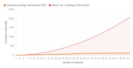
Cumulative Cost: Dynamic Array vs Naïve Fixed Array
5. How to apply amortised analysis yourself
Seeing the technique in a textbook is one thing; applying it to a new data structure you are designing is another. Fortunately, there is a repeatable process you can follow.
First, identify the costly operations. Ask yourself which operations, in the worst case, do work proportional to the current size of the structure. These are your resize, rebuild, or rebalance events.
Second, ask whether those operations are rate-limited. Can the expensive event happen on every operation, or does some structural property prevent it? If it cannot happen consecutively — because it resets the condition that caused it — you have the hallmark of amortised behaviour.
Third, choose a potential function or accounting scheme. A potential function should be zero (or minimal) right after an expensive operation, and should grow with the accumulated “debt” the structure is carrying. If you are using the accounting method, ask: how much credit does each cheap operation need to save in order to pay for the next expensive one?
Finally, verify that the credit or potential never goes negative. This is the formal condition that makes the analysis sound. If it ever goes negative, your function is not valid — go back and adjust.
Confusing amortised O(1) with guaranteed O(1). If your application is latency-sensitive (think real-time systems, game engines, financial trading), a single O(n) spike — even a rare one — may be unacceptable. In those cases, consider structures with hard per-operation bounds, like a circular buffer with pre-allocated capacity.
6. Amortised vs average-case: do not confuse them
This distinction trips up a surprising number of experienced developers. Average-case analysis assumes something about the distribution of inputs or the randomness of operations. Amortised analysis assumes nothing — it is a worst-case guarantee, just over a sequence rather than a single operation.
For example, a randomised hash table (using a random hash function) can give expected O(1) lookup in the average case, because collisions are unlikely on average. But a deterministic hash table with a poor hash function can degrade to O(n) if the inputs are adversarial. Amortised analysis would never make a probabilistic claim like that; it would instead say: over any sequence of n operations, the total cost is at most cn for some constant c.
In practice, it is common to see bounds that combine both. Skip lists, for instance, are O(log n) expected with high probability — average-case with tight probabilistic bounds. Fibonacci heaps are O(1) amortised — worst-case over sequences. These are fundamentally different kinds of guarantees, and reading them interchangeably leads to incorrect performance models.
7. What we have learned
- Amortised analysis lets you reason about the total cost of a sequence of operations, not just the worst-case cost of a single one — giving a tighter, often more truthful bound.
- Three standard methods exist — aggregate, accounting, and potential — all of which give consistent results from different perspectives.
- Dynamic arrays achieve O(1) amortised insert through a doubling strategy: cheap inserts accumulate credit that pays for rare, expensive resizes.
- Hash tables, Union-Find, splay trees, and Fibonacci heaps all rely on amortised analysis for their headline complexity guarantees.
- Amortised analysis is a worst-case bound on sequences — it is fundamentally different from average-case analysis, which involves probabilistic assumptions.
- For latency-sensitive applications, amortised guarantees may not be sufficient; the distinction between “fast on average” and “never slow” matters in production.
