Editor’s note: This is a post by Apache Flink PMC members Fabian Hueske and Kostas Tzoumas. Fabian and Kostas are also co-founders of data Artisans.
A very large part of today’s data processing is done on data that is continuously produced, e.g., data from user activity logs, web logs, machines, sensors, and database transactions. Until now, data streaming technology was lacking in several areas, such as performance, correctness, and operability, forcing users to roll their own applications to ingest and analyze these continuous data streams, or (ab)use batch processing tools to simulate continuous ingestion and analysis pipelines.
This is no longer the case, as streaming technology has now matured and is being rapidly adopted by the enterprise. Writing data applications on top of streaming data has several benefits:
- It decreases the overall latency, as data does not have to be necessarily moved to a filesystem or a database before becoming valuable for analytics.
- It simplifies the architecture of data infrastructure, as there are far fewer moving parts to be maintained and coordinated to ensure timely answers from data signals.
- It makes the time dimension explicit, associating each data record with its timestamp, and allowing analytics to process and group events based on these timestamps.
Overall, streaming technology enables the obvious: continuous processing on data that is naturally produced by continuous real-world sources (which is most “big” data sets).
Apache Flink is an open source distributed platform for stream and batch processing with a long history of innovation, and a top-level project of the Apache Software Foundation with a community of more than 150 contributors. In this post, we focus on the stream processing capabilities of the system. Flink 0.10, the latest release of Apache Flink and a result of the work of about 80 individuals, has brought a number of new features that make Flink stand out as a stream processing system in the open source space.
- Support for event time and out of order streams: In reality, streams of events rarely arrive in the order that they are produced, especially streams from distributed systems and devices. Until now, it was up to the application programmer to correct this “time drift,” or simply ignore it and accept inaccurate results, as streaming systems (at least in the open source) had no support for event time. Flink 0.10 is the first open source engine that supports out of order streams and event time.
- Expressive and easy-to-use APIs in Scala and Java: Flink’s DataStream API ports many operators which are well known from batch processing APIs such as map, reduce, and join. In addition, it provides stream-specific operations such as window, split, and connect. First-class support for user-defined functions eases the implementation of custom application behavior. The DataStream API is available in Scala and Java.
- Support for sessions and unaligned windows: Most streaming systems have some concept of windowing, i.e., a grouping of events based on some function of time. Unfortunately, in many systems these windows are hard-coded and connected with the system’s internal checkpointing mechanism. Flink is the first open source streaming engine that completely decouples windowing from fault tolerance, allowing for richer forms of windows, such as sessions.
- Consistency, fault tolerance, and high availability: Flink guarantees consistent state updates in the presence of failures (often called “exactly-once processing”), and consistent data movement between selected sources and sinks (e.g., consistent data movement between Kafka and HDFS). Flink also supports master failover, eliminating any single point of failure.
- Low latency and high throughput: We have clocked Flink at 1.5 million events per second per core, and have also observed latencies in the 25 millisecond range for jobs that include network data shuffling. Using a tuning knob, Flink users can navigate the latency-throughput tradeoff, making the system suitable for both high-throughput data ingestion and transformations, as well as ultra low latency (millisecond range) applications.
- Integration: Flink integrates with a wide variety of open source systems for data input and output (e.g., HDFS, Kafka, Elasticsearch, HBase, and others), deployment (e.g., YARN), as well as acting as an execution engine for other frameworks (e.g., Cascading, Apache Beam incubating aka Google Cloud Dataflow). The Flink project itself comes bundled with a Hadoop MapReduce compatibility layer, a Storm compatibility layer, as well as libraries for machine learning and graph processing.
- Support for batch: In Flink, batch processing is a special case of stream processing, as finite data sources are just streams that happen to end. Flink offers a full toolset for batch processing with a dedicated DataSet API and libraries for machine learning and graph processing. In addition, Flink contains several batch-specific optimizations (e.g., for scheduling, memory management, and query optimization), matching and even out-performing dedicated batch processing engines in batch use cases.
- Developer productivity and operational simplicity: Flink runs in a variety of environments. Local execution within an IDE significantly eases development and debugging of Flink applications. In distributed setups, Flink runs at massive scale-out. The YARN mode allows users to bring up Flink clusters in a matter of seconds. Flink serves monitoring metrics of jobs and the system as a whole via a well-defined REST interface. A build-in web dashboard displays these metrics and makes monitoring of Flink very convenient.
Flink in the Data Infrastructure Stack
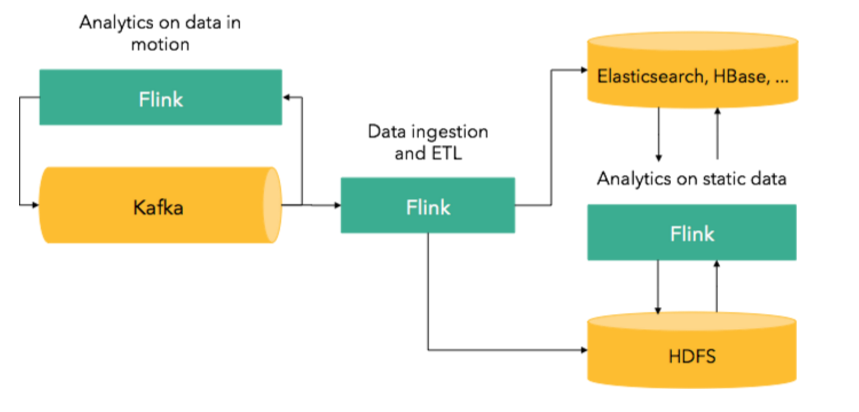
Flink is a storage-agnostic stream processing framework, and is thus used in conjunction with data storage or brokering systems. A typical architectural pattern is to use Flink in conjunction with Apache Kafka to:
- Ingest data into other systems such as HDFS, databases, or search indices and create continuous ETL pipelines.
- Perform analytics directly on the moving data to create alerts, dashboards, or power operational applications obviating the need for ingestion and ETL.
- Perform machine learning on streams by continuously building models of the events as they arrive and using the model to serve online recommendations.
Since Flink is a full-fledged system for batch processing as well, it can also be used for applications on top of static data. The following picture provides an overview of where Flink applications might fit in a broader stack:
We have seen Flink being used for a variety of use cases, such as monitoring of equipment, analysis of machine-generated logs, analytics on customer activity data, online recommender systems, and graph processing applications. Check out the talks from this year’s Flink Forward for an overview of how companies are using Flink.
Hands-on Stream Processing with Flink
Now that you understand Apache Flink’s stream processing features, it’s time to take a look at the capabilities of its DataStream API and learn about three example applications. We share fully-packaged Scala implementations of these examples on Github and encourage you to run these programs in your IDE and play with the code. All you have to do is to follow the instructions posted at the repository, which will guide you to import the code in your IDE, run an example application from your IDE, and track execution progress with Flink’s web dashboard.
Our demo applications process a stream of taxi ride events that originate from a public dataset of the New York City Taxi and Limousine Commission (TLC). The data set consists of records about taxi trips in New York City from 2009 to 2015. We took some of this data and converted it into a data set of taxi ride events by splitting each trip record into a ride start and a ride end event. The events have the following schema:
rideId: Long // unique id for each ride
time: DateTime // timestamp of the start/end event
isStart: Boolean // true = ride start, false = ride end
location: GeoPoint // lon/lat of pick-up/drop-off location
passengerCnt: short // number of passengers
travelDist: float // total travel distance, -1 on start events
We have implemented a custom SourceFunction to serve a DataStream[TaxiRide] from the ride event data set. In order to generate the stream as realistically as possible, events are emitted by their timestamps. Two events that occurred ten minutes after each other in reality are served ten minutes apart. A speed-up factor can be specified to “fast-forward” the stream, i.e., with a speed-up factor of two, the events are served five minutes apart. Moreover, we can specify a maximum serving delay which causes events to be randomly delayed within the bound to simulate an out-of-order stream. All examples operate in event-time mode. This guarantees consistent results even in case of historic data or data which is delivered out of order. Note that out-of-order streams are very common in real-world applications, especially if events originate from several sources such as distributed sensor networks.
Identify popular locations
For our first demo application, we want to identify locations in New York City to which many people arrive by taxi. We implemented this application as TotalArrivalCount.scala and will guide you step-by-step through the program.
First, we obtain a StreamExecutionEnvironment and set the TimeCharacteristic to EventTime. Event time processing guarantees that the program computes consistent results even if events arrive out of order at the stream processor.
val env: StreamExecutionEnvironment = DemoStreamEnvironment.env
env.setStreamTimeCharacteristic(TimeCharacteristic.EventTime)
Next, we define a data source that generates a DataStream[TaxiRide] with at most 60 seconds serving delay (events are out of order by max. 1 minute) and a speed-up factor of 600 (events that occurred in 10 minutes are served within 1 second).
// Define the data source
val rides: DataStream[TaxiRide] = env.addSource(new TaxiRideSource(
  “./data/nycTaxiData.gz”, 60, 600.0f))
Since we are only interested in locations that people travel to (and not where they come from) and because the data is little bit messy (locations are not always correctly specified), we apply a few filters first to cleanse the data.
val cleansedRides = rides
  // filter for trip end events
  .filter( !_.isStart )
  // filter for events in NYC
  .filter( r => NycGeoUtils.isInNYC(r.location) )
The taxi ride stream defines event locations as coordinates with continuous longitude/latitude values. We need to map them into a finite set of regions in order to be able to aggregate events by location. We do this by defining a grid of approximately 100×100 meter cells on the area of New York City. We use a utility class (NycGeoUtils.scala) to map event locations to cell ids and extract the event timestamp and passenger count as follows:
// map location coordinates to cell Id, timestamp, and passenger count
val cellIds: DataStream[(Int, Long, Short)] = cleansedRides
.map { r =>
  ( NycGeoUtils.mapToGridCell(r.location), r.time.getMillis, r.passengerCnt )
}
After these preparation steps, we have the data that we would like to aggregate. Since we want to compute the passenger count for each location (cell id), we start by keying the stream by cell id (_._1). This will basically organize and partition the stream by cell id. Subsequently, we apply a fold transformation on each key partition to compute the sum of all passengers and the latest timestamp. The fold transformation starts with an initial value of (0, 0, 0) and computes the sum by adding one record at a time. Since the fold function aggregates an infinite stream, it returns the current aggregation value for each input record, i.e., it sends out an updated count.
val passengerCnts: DataStream[(Int, Long, Int)] = cellIds
  // key stream by cell Id
  .keyBy(_._1)
  // sum passengers per cell Id and update time
  .fold((0, 0L, 0), (s: (Int, Long, Int), r: (Int, Long, Short)) =>
    { (r._1, s._2.max(r._2), s._3 + r._3) } )
Finally, we translate the cell id back into a GeoPoint (which is the center of the cell), print the result stream to the standard output, and start executing the program.
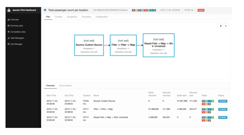
val cntByLocation: DataStream[(Int, Long, GeoPoint, Int)] = passengerCnts
  // map cell Id back to GeoPoint
  .map( r => (r._1, r._2, NycGeoUtils.getGridCellCenter(r._1), r._3 ) )

cntByLocation
  // print to console
  .print()

env.execute(“Total passenger count per location”)
When you execute the TotalArrivalCount.scala program in your IDE, you will see log messages for initializing the program, scheduling its operators, and starting the processing of the data stream as well as the output of the program being printed to the standard output. Flink will also start its web dashboard that you can access by opening http://localhost:8081 in your browser. The dashboard shows many monitoring statistics of running programs and the system as a whole, helps to analyze the behavior of finished jobs, and provides access to configuration and log files. The following screenshot shows the job execution overview of the dashboard.
Identify the popular locations of the last 15 minutes
Our first demo application computes for each location the total number of people that arrived by taxi. While this helps to identify places that are popular in general, it also hides a lot of information such as variations over time. For our next example, we identify places that are popular within a certain period of time, i.e., we compute every 5 minutes the number of passengers that arrived at each location within the last 15 minutes by taxi. This is kind of computation is known as a sliding window operation.
The basic structure of our sliding window program SlidingArrivalCount.scala is very similar to the program of our first example. We cleanse the stream and map the location coordinates to a cell id and extract the passenger count. Once we have that, we again key the stream by cell id as before but instead of applying a fold operator on the keyed stream, we define a sliding time window and run a WindowFunction by calling apply():
val passengerCnts: DataStream[(Int, Long, Int)] = cellIds
  // key stream by cell Id
  .keyBy(_._1)
  // define sliding window on keyed streams
  .timeWindow(Time.minutes(15), Time.minutes(5))
  // count events in window
  .apply { (
    cell: Int,
    window: TimeWindow,
    events: Iterable[(Int, Short)],
    out: Collector[(Int, Long, Int)]) =>
      out.collect( ( cell, window.getEnd, events.map( _._2 ).sum ) )
  }
The timeWindow() operation groups the events of the stream into finite sets of records on which a window or aggregation function can be applied. In our example, we call apply() to process the windows using a WindowFunction. The WindowFunction receives four parameters, a Tuple that contains the key of the window, a TimeWindow object that contains details such as the start and end time of the window, an Iterable over all elements in the window, and a Collector to collect the records emitted by the WindowFunction. We want to count the number of passengers that arrive within the time defined by the window. Therefore, we have to emit a single record that contains the grid cell id, the end time of the window, and the sum of the ride passenger counts which is computed by extracting the individual passenger counts from the Iterable (events.map( _._2)) and summing them (.sum).
Finally, we map the grid cell back to a GeoPoint as before and print the resulting stream. This program will produce every five minutes one record for each location that received at least one taxi passenger. Note that in event time processing, time windows are synchronized, i.e., the windows of all keys are evaluated at the same logical time.
Compute early counts for popular locations
The sliding window demo application computes every 5 minutes the arrival counts for each location of the last 15 minutes. However, certain applications may require more timely information to allow for immediate response such as generating an alert. For our last example, we want to compute sliding window counts as in our previous example, but in addition we want to receive an early count whenever a multiple of 50 persons arrived at a location within the time bounds of a window (15 minutes), i.e., we would like to get partial counts for a window when its arrival count exceeds 50, 100, 150, and so on.
Flink’s DataStream API offers a Trigger interface to precisely control when a window is evaluated, i.e., when the window function is called. Our last example program EarlyArrivalCount.scala, reuses the code to cleanse the stream and to assign cell ids to events as before. Here we only show the code to compute the partial and final arrival counts:
val passengerCnts: DataStream[(Int, Long, Int)] = cellIds
  // key stream by cell Id
  .keyBy( _._1 )
  // define sliding window on keyed streams
  .timeWindow(Time.mintes(15), Time.minutes(5))
  .trigger(new EarlyCountTrigger(50))
  // count events in window
  .apply( (cell, window, events, out: Collector[(Int, Long, Int)]) => {
    out.collect((cell, window.getEnd, events.map( _._2 ).sum ))
  })
Comparing this code snippet to the code of the sliding window example (SlidingArrivalCount.scala), we see that the keyBy(), timeWindow() , and apply() statements are exactly as before. There is only one difference, namely the line that defines our custom trigger. By defining a custom trigger, we overwrite the default trigger of the time window which would evaluate the window (call the window function) at the end of its defined time frame.
The Trigger interface of the DataStream API defines three methods:
onElement(), which is called for each element that enters a window.onEventTime(), which is called when a previously registered event time timer expires.onProcessingTime(), which is called when a previously registered processing time trigger expires.
Our custom trigger implementation EarlyCountTrigger implements these methods as follows:
override def onElement(
  event: (Int, Short),
  timestamp: Long,
  window: TimeWindow,
  ctx: TriggerContext): TriggerResult = {

  // register event time timer for end of window
  ctx.registerEventTimeTimer(window.getEnd)

  // get current count
  val personCnt = ctx.getKeyValueState[Integer]("personCnt", 0)
  // update count by passenger cnt of new event
  personCnt.update(personCnt.value() + event._2)
  // check if count is high enough for early notification
  if (personCnt.value() < triggerCnt) {
    // not there yet
    TriggerResult.CONTINUE
  }
  else {
    // trigger count is reached
    personCnt.update(0)
    TriggerResult.FIRE
  }
}
The onElement() method of our custom trigger first registers an event time timer for the defined end time of the window. This timer ensures that the onEventTime() method is called at the end of the window times to compute the final result. Next, we obtain the state of the trigger which is a simple Integer that holds the current passenger count. We use Flink’s interface for managed state at this point to ensure that the state of the trigger is periodically checkpointed and consistently restored in case of a failure. Then we update the passenger count state by the count of the event which was added to the window and check if the threshold is exceeded. If this is not the case, TriggerResult.CONTINUE is returned to signal that processing continues. If the threshold is exceeded, we reset the count state to zero and return TriggerResult.FIRE which causes the window function to evaluate the window (Note: FIRE does not remove the elements from the window).
override def onEventTime(
  time: Long,
  window: TimeWindow,
  ctx: TriggerContext): TriggerResult = {

  // trigger final computation
  TriggerResult.FIRE_AND_PURGE
}
Once the event time passes the end time of the window, the onEventTime() method is called which returns the TriggerResult.FIRE_AND_PURGE to compute the final window result and finally purge all elements from the window.
The onProcessingTime() method is not implemented, because we are operating in event time mode and do not register a processing time timer in our trigger.
By defining a sliding window and our custom trigger, we implement the desired behavior of our last demo application. The program computes sliding window counts but emits partial counts if certain thresholds are exceeded. The partial counts are constantly updated by newer partial counts and eventually by the final count.
Time windows and triggers are not the only concepts supported by Flink’s DataStream API to group stream events. In addition to the Trigger interface, the DataStream API offers an Evictor interface to remove elements from the beginning of a window before it is evaluated. Moreover, you can define CountWindows which evaluate window functions based on event counts and GlobalWindows which collect all data and put you in charge of defining trigger policies and evicting elements. With windows, triggers, evictors, and window functions at hand, you have a very expressive toolbox to precisely define custom window logic for your stream processing applications.
Visualizing data streams with Kibana
Flink offers several connectors to write data streams to storage systems such as Apache Kafka, HDFS, and Elasticsearch. You might have noticed that our demo applications contain code to write the computed location arrival counts into an Elasticsearch. Once the data is in Elasticsearch, we can use Kibana, a dashboard to visualize data stored in Elasticsearch, to plot the location counts on a map and to analyze the results of our programs. The following screenshot shows how Kibana visualizes the result of the streaming program that computes popular locations in New York City.
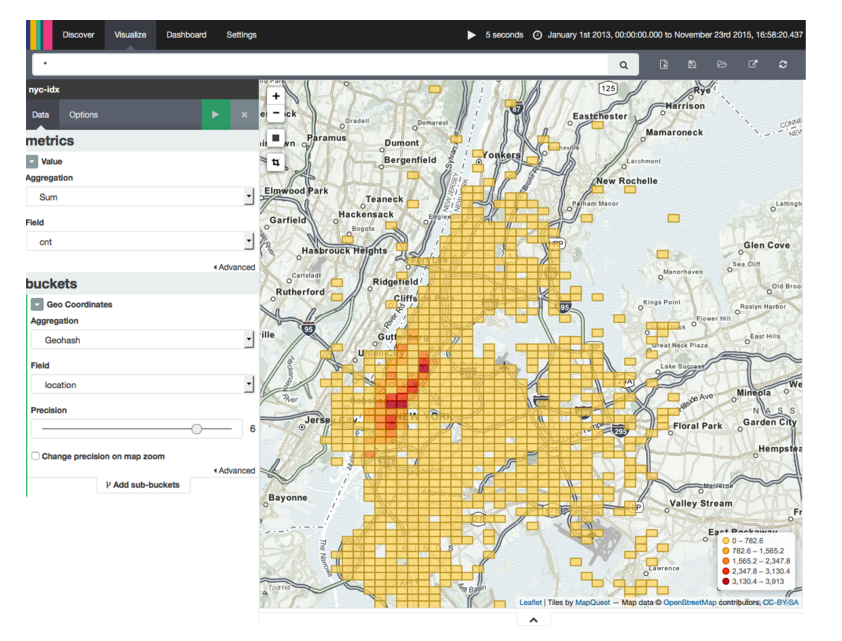
We provide detailed setup instructions for Elasticsearch and Kibana on our Github repository. Check it out if you would like to play with Flink, Elasticsearch, and Kibana.
Wrapping Up
Apache Flink is a production-ready distributed stream processor with a competitive feature set. Support for out-of-order event streams, event time processing, and its very flexible windowing mechanics make Flink stand out in the space of open source stream processing solutions. In this blog post, we presented three demo applications and showcased the expressive power of windows in Flink’s DataStream API. The code is available on Github, and we invite you to import the examples into your IDE to play around and explore Flink yourself.
From an enterprise architecture viewpoint as exemplified by the Zeta architecture, Flink can serve as a flexible computation engine for a very large variety of data formats. Flink can read data from a variety of data sources, such as distributed filesystems (including HDFS, MapR-FS, and all HDFS-compatible file systems), databases (such as HBase and MapR-DB), and message queues (such as MapR Streams and Kafka). Flink can currently run on YARN and on Mesos using Myriad, and there is an ongoing effort to make Flink run natively on Mesos. Finally, Flink can act as a computation engine for other APIs as well. Currently, Flink ships with a compatibility layer for Apache Storm, and there are runners for Dataflow (the newly proposed Apache Beam project) on Flink and Cascading on Flink.
About the authors:

Fabian Hueske is a PMC member of Apache Flink. He has been contributing to Flink since its earliest days when it started as a research project as part of his PhD studies at TU Berlin. Fabian did internships with IBM Research, SAP Research, and Microsoft Research and is a co-founder of data Artisans.
Kostas Tzoumas:

Kostas Tzoumas is co-founder and CEO of data Artisans, a company created by the original creators of the Apache Flink framework, and a PMC member of Apache Flink. Before founding data Artisans, Kostas was a postdoctoral researcher at TU Berlin, with Microsoft Research, and Aalborg University.
| Reference: | The Essential Guide to Streaming-first Processing with Apache Flink from our JCG partner Fabian Hueske at the Mapr blog. |
