R: Wimbledon – How do the seeds get on?

Mark NeedhamJuly 7th, 2015Last Updated: July 6th, 2015

0 18 5 minutes read

Continuing on with the Wimbledon data set I’ve been playing with I wanted to do some exploration on how the seeded players have fared over the years.

Taking the last 10 years worth of data there have always had 32 seeds and with the following function we can feed in a seeding and get back the round they would be expected to reach:

expected_round = function(seeding) {  
  if(seeding == 1) {
    return("Winner")
  } else if(seeding == 2) {
    return("Finals") 
  } else if(seeding <= 4) {
    return("Semi-Finals")
  } else if(seeding <= 8) {
    return("Quarter-Finals")
  } else if(seeding <= 16) {
    return("Round of 16")
  } else {
    return("Round of 32")
  }
}
 
> expected_round(1)
[1] "Winner"
 
> expected_round(4)
[1] "Semi-Finals"

We can then have a look at each of the Wimbledon tournaments and work out how far they actually got.

round_reached = function(player, main_matches) {
  furthest_match = main_matches %>% 
    filter(winner == player | loser == player) %>% 
    arrange(desc(round)) %>% 
    head(1)  
 
    return(ifelse(furthest_match$winner == player, "Winner", as.character(furthest_match$round)))
}
 
seeds = function(matches_to_consider) {
  winners =  matches_to_consider %>% filter(!is.na(winner_seeding)) %>% 
    select(name = winner, seeding =  winner_seeding) %>% distinct()
  losers = matches_to_consider %>% filter( !is.na(loser_seeding)) %>% 
    select(name = loser, seeding =  loser_seeding) %>% distinct()
 
  return(rbind(winners, losers) %>% distinct() %>% mutate(name = as.character(name)))
}

Let’s have a look how the seeds got on last year:

matches_to_consider = main_matches %>% filter(year == 2014)
 
result = seeds(matches_to_consider) %>% group_by(name) %>% 
    mutate(expected = expected_round(seeding), round = round_reached(name, matches_to_consider)) %>% 
    ungroup() %>% arrange(seeding)
 
rounds = c("Did not enter", "Round of 128", "Round of 64", "Round of 32", "Round of 16", "Quarter-Finals", "Semi-Finals", "Finals", "Winner")
result$round = factor(result$round, levels = rounds, ordered = TRUE)
result$expected = factor(result$expected, levels = rounds, ordered = TRUE) 
 
> result %>% head(10)
Source: local data frame [10 x 4]
 
             name seeding       expected          round
1  Novak Djokovic       1         Winner         Winner
2    Rafael Nadal       2         Finals    Round of 16
3     Andy Murray       3    Semi-Finals Quarter-Finals
4   Roger Federer       4    Semi-Finals         Finals
5   Stan Wawrinka       5 Quarter-Finals Quarter-Finals
6   Tomas Berdych       6 Quarter-Finals    Round of 32
7    David Ferrer       7 Quarter-Finals    Round of 64
8    Milos Raonic       8 Quarter-Finals    Semi-Finals
9      John Isner       9    Round of 16    Round of 32
10  Kei Nishikori      10    Round of 16    Round of 16

We’ll wrap all of that code into the following function:

expectations = function(y, matches) {
  matches_to_consider = matches %>% filter(year == y)  
 
  result = seeds(matches_to_consider) %>% group_by(name) %>% 
    mutate(expected = expected_round(seeding), round = round_reached(name, matches_to_consider)) %>% 
    ungroup() %>% arrange(seeding)
 
  result$round = factor(result$round, levels = rounds, ordered = TRUE)
  result$expected = factor(result$expected, levels = rounds, ordered = TRUE)  
 
  return(result)
}

Next, instead of showing the round names it’d be cool to come up with numerical value indicating how well the player did:

-1 would mean they lost in the round before their seeding suggested e.g. seed 2 loses in Semi Final
2 would mean they got 2 rounds further than they should have e.g. Seed 7 reaches the Final

The unclass function comes to our rescue here:

# expectations plot
years = 2005:2014
exp = data.frame()
for(y in years) {
  differences = (expectations(y, main_matches)  %>% 
                   mutate(expected_n = unclass(expected), 
                          round_n = unclass(round), 
                          difference = round_n - expected_n))$difference %>% as.numeric()    
  exp = rbind(exp, data.frame(year = rep(y, length(differences)), difference = differences)) 
}
 
> exp %>% sample_n(10)
Source: local data frame [10 x 6]
 
              name seeding expected_n round_n difference year
1    Tomas Berdych       6          6       5         -1 2011
2    Tomas Berdych       7          6       6          0 2013
3     Rafael Nadal       2          8       5         -3 2014
4    Fabio Fognini      16          5       4         -1 2014
5  Robin Soderling      13          5       5          0 2009
6    Jurgen Melzer      16          5       5          0 2010
7  Nicolas Almagro      19          4       2         -2 2010
8    Stan Wawrinka      14          5       3         -2 2011
9     David Ferrer       7          6       5         -1 2011
10 Mikhail Youzhny      14          5       5          0 2007

We can then group by the ‘difference’ column to see how seeds are getting on as a whole:

> exp %>% count(difference)
Source: local data frame [9 x 2]
 
  difference  n
1         -5  2
2         -4  7
3         -3 24
4         -2 70
5         -1 66
6          0 85
7          1 43
8          2 17
9          3  4
 
library(ggplot2)
ggplot(aes(x = difference, y = n), data = exp %>% count(difference)) +
  geom_bar(stat = "identity") +
  scale_x_continuous(limits=c(min(potential), max(potential) + 1))

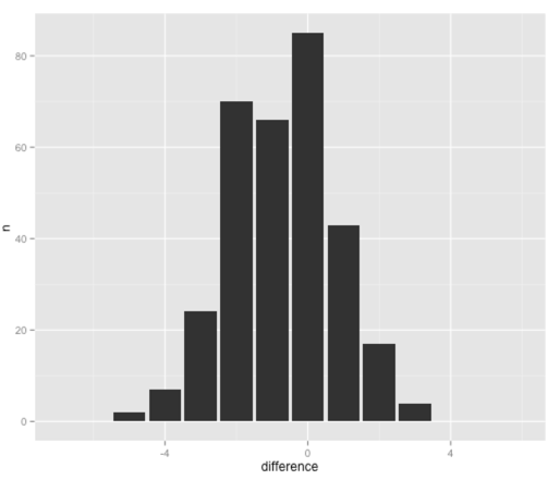
So from this visualisation we can see that the most common outcome for a seed is that they reach the round they were expected to reach. There are still a decent number of seeds who do 1 or 2 rounds worse than expected as well though.

Antonios suggested doing some analysis of how the seeds fared on a year by year basis – we’ll start by looking at what % of them exactly achieved their seeding:

exp$correct_pred = 0
exp$correct_pred[dt$difference==0] = 1
 
exp %>% group_by(year) %>% 
  summarise(MeanDiff = mean(difference),
            PrcCorrect = mean(correct_pred),
            N=n())
 
Source: local data frame [10 x 4]
 
   year   MeanDiff PrcCorrect  N
1  2005 -0.6562500  0.2187500 32
2  2006 -0.8125000  0.2812500 32
3  2007 -0.4838710  0.4193548 31
4  2008 -0.9677419  0.2580645 31
5  2009 -0.3750000  0.2500000 32
6  2010 -0.7187500  0.4375000 32
7  2011 -0.7187500  0.0937500 32
8  2012 -0.7500000  0.2812500 32
9  2013 -0.9375000  0.2500000 32
10 2014 -0.7187500  0.1875000 32

Some years are better than others – we can use a chisq test to see whether there are any significant differences between the years:

tbl = table(exp$year, exp$correct_pred)
tbl
 
> chisq.test(tbl)
 
	Pearson's Chi-squared test
 
data:  tbl
X-squared = 14.9146, df = 9, p-value = 0.09331

This looks for at least one statistically significant different between the years, although it doesn’t look like there are any. We can also try doing a comparison of each year against all the others:

> pairwise.prop.test(tbl)
 
	Pairwise comparisons using Pairwise comparison of proportions 
 
data:  tbl 
 
     2005 2006 2007 2008 2009 2010 2011 2012 2013
2006 1.00 -    -    -    -    -    -    -    -   
2007 1.00 1.00 -    -    -    -    -    -    -   
2008 1.00 1.00 1.00 -    -    -    -    -    -   
2009 1.00 1.00 1.00 1.00 -    -    -    -    -   
2010 1.00 1.00 1.00 1.00 1.00 -    -    -    -   
2011 1.00 1.00 0.33 1.00 1.00 0.21 -    -    -   
2012 1.00 1.00 1.00 1.00 1.00 1.00 1.00 -    -   
2013 1.00 1.00 1.00 1.00 1.00 1.00 1.00 1.00 -   
2014 1.00 1.00 1.00 1.00 1.00 1.00 1.00 1.00 1.00
 
P value adjustment method: holm

2007/2011 and 2010/2011 show the biggest differences but they’re still not significant. Since we have so few data items in each bucket there has to be a really massive difference for it to be significant.