I recently came across an excellent article written by Stian Haklev in which he describes things he wishes he’d been told before starting out with R, one being to do all data clean up in code which I thought I’d give a try.
My goal is to leave the raw data completely unchanged, and do all the transformation in code, which can be rerun at any time.
While I’m writing the scripts, I’m often jumping around, selectively executing individual lines or code blocks, running commands to inspect the data in the REPL (read-evaluate-print-loop, where each command is executed as soon as you type enter, in the picture above it’s the pane to the right), etc.
But I try to make sure that when I finish up, the script is runnable by itself.
I thought the Google Trends data set would be an interesting one to play around with as it gives you a CSV containing several different bits of data of which I’m only interested in ‘interest over time’.
It’s not very easy to automate the download of the CSV file so I did that bit manually and automated everything from there onwards.
The first step was to read the CSV file and explore some of the rows to see what it contained:
> library(dplyr)

> googleTrends = read.csv("/Users/markneedham/Downloads/report.csv", row.names=NULL)

> googleTrends %>% head()
##                   row.names Web.Search.interest..neo4j
## 1 Worldwide; 2004 - present
## 2        Interest over time
## 3                      Week                      neo4j
## 4   2004-01-04 - 2004-01-10                          0
## 5   2004-01-11 - 2004-01-17                          0
## 6   2004-01-18 - 2004-01-24                          0

> googleTrends %>% sample_n(10)
##                   row.names Web.Search.interest..neo4j
## 109 2006-01-08 - 2006-01-14                          0
## 113 2006-02-05 - 2006-02-11                          0
## 267 2009-01-18 - 2009-01-24                          0
## 199 2007-09-30 - 2007-10-06                          0
## 522 2013-12-08 - 2013-12-14                         88
## 265 2009-01-04 - 2009-01-10                          0
## 285 2009-05-24 - 2009-05-30                          0
## 318 2010-01-10 - 2010-01-16                          0
## 495 2013-06-02 - 2013-06-08                         79
## 28  2004-06-20 - 2004-06-26                          0

> googleTrends %>% tail()
##                row.names Web.Search.interest..neo4j
## 658        neo4j example                   Breakout
## 659 neo4j graph database                   Breakout
## 660           neo4j java                   Breakout
## 661           neo4j node                   Breakout
## 662           neo4j rest                   Breakout
## 663       neo4j tutorial                   Breakout
We only want to keep the rows which contain (week, interest) pairs so the first thing we’ll do is rename the columns:
names(googleTrends) = c("week", "score")Now we want to strip out the rows which don’t contain (week, interest) pairs. The easiest way to do this is to look for rows which don’t contain date values in the ‘week’ column.
First we need to split the start and end dates in that column by using the strsplit function.
I found it much easier to apply the function to each row individually rather than passing in a list of values so I created a dummy column with a row number in to allow me to do that (a trick Antonios showed me):
> googleTrends %>%
    mutate(ind = row_number()) %>%
    group_by(ind) %>%
    mutate(dates = strsplit(week, " - "),
           start = dates[[1]][1] %>% strptime("%Y-%m-%d") %>% as.character(),
           end =   dates[[1]][2] %>% strptime("%Y-%m-%d") %>% as.character()) %>%
    head()
## Source: local data frame [6 x 6]
## Groups: ind
##
##                        week score ind    dates      start        end
## 1 Worldwide; 2004 - present     1   1 <chr[2]>         NA         NA
## 2        Interest over time     1   2 <chr[1]>         NA         NA
## 3                      Week    90   3 <chr[1]>         NA         NA
## 4   2004-01-04 - 2004-01-10     3   4 <chr[2]> 2004-01-04 2004-01-10
## 5   2004-01-11 - 2004-01-17     3   5 <chr[2]> 2004-01-11 2004-01-17
## 6   2004-01-18 - 2004-01-24     3   6 <chr[2]> 2004-01-18 2004-01-24
Now we need to get rid of the rows which have an NA value for ‘start’ or ‘end’:
> googleTrends %>%
    mutate(ind = row_number()) %>%
    group_by(ind) %>%
    mutate(dates = strsplit(week, " - "),
           start = dates[[1]][1] %>% strptime("%Y-%m-%d") %>% as.character(),
           end =   dates[[1]][2] %>% strptime("%Y-%m-%d") %>% as.character()) %>%
    filter(!is.na(start) | !is.na(end)) %>%
    head()
## Source: local data frame [6 x 6]
## Groups: ind
##
##                      week score ind    dates      start        end
## 1 2004-01-04 - 2004-01-10     3   4 <chr[2]> 2004-01-04 2004-01-10
## 2 2004-01-11 - 2004-01-17     3   5 <chr[2]> 2004-01-11 2004-01-17
## 3 2004-01-18 - 2004-01-24     3   6 <chr[2]> 2004-01-18 2004-01-24
## 4 2004-01-25 - 2004-01-31     3   7 <chr[2]> 2004-01-25 2004-01-31
## 5 2004-02-01 - 2004-02-07     3   8 <chr[2]> 2004-02-01 2004-02-07
## 6 2004-02-08 - 2004-02-14     3   9 <chr[2]> 2004-02-08 2004-02-14
Next we’ll get rid of ‘week’, ‘ind’ and ‘dates’ as we aren’t going to need those anymore:
> cleanGoogleTrends = googleTrends %>%
    mutate(ind = row_number()) %>%
    group_by(ind) %>%
    mutate(dates = strsplit(week, " - "),
           start = dates[[1]][1] %>% strptime("%Y-%m-%d") %>% as.character(),
           end =   dates[[1]][2] %>% strptime("%Y-%m-%d") %>% as.character()) %>%
    filter(!is.na(start) | !is.na(end)) %>%
    ungroup() %>%
    select(-c(ind, dates, week))

> cleanGoogleTrends %>% head()
## Source: local data frame [6 x 3]
##
##   score      start        end
## 1     3 2004-01-04 2004-01-10
## 2     3 2004-01-11 2004-01-17
## 3     3 2004-01-18 2004-01-24
## 4     3 2004-01-25 2004-01-31
## 5     3 2004-02-01 2004-02-07
## 6     3 2004-02-08 2004-02-14

> cleanGoogleTrends %>% sample_n(10)
## Source: local data frame [10 x 3]
##
##    score      start        end
## 1      8 2010-09-26 2010-10-02
## 2     73 2013-11-17 2013-11-23
## 3     52 2012-07-01 2012-07-07
## 4      3 2005-06-19 2005-06-25
## 5      3 2004-12-12 2004-12-18
## 6      3 2009-09-06 2009-09-12
## 7     71 2014-09-14 2014-09-20
## 8      3 2004-12-26 2005-01-01
## 9     62 2013-03-03 2013-03-09
## 10     3 2006-03-19 2006-03-25

> cleanGoogleTrends %>% tail()
## Source: local data frame [6 x 3]
##
##   score      start        end
## 1    80 2014-10-19 2014-10-25
## 2    80 2014-10-26 2014-11-01
## 3    84 2014-11-02 2014-11-08
## 4    81 2014-11-09 2014-11-15
## 5    83 2014-11-16 2014-11-22
## 6     2 2014-11-23 2014-11-29
Ok now we’re ready to plot. This was my first attempt:
> library(ggplot2)
> ggplot(aes(x = start, y = score), data = cleanGoogleTrends) +
    geom_line(size = 0.5)
## geom_path: Each group consist of only one observation. Do you need to adjust the group aesthetic?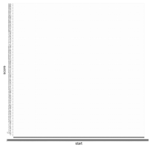
As you can see, not too successful! The first mistake I’ve made is not telling ggplot that the ‘start’ column is a date and so it can use that ordering when plotting:
> cleanGoogleTrends = cleanGoogleTrends %>% mutate(start =  as.Date(start))
> ggplot(aes(x = start, y = score), data = cleanGoogleTrends) +
    geom_line(size = 0.5)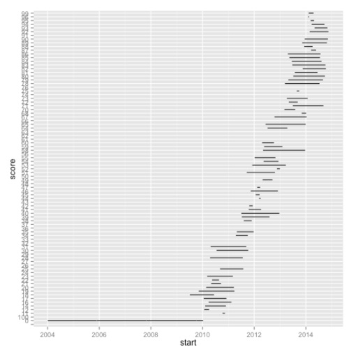
My next mistake is that ‘score’ is not being treated as a continuous variable and so we’re ending up with this very strange looking chart. We can see that if we call the class function:
> class(cleanGoogleTrends$score)
## [1] "factor"
Let’s fix that and plot again:
> cleanGoogleTrends = cleanGoogleTrends %>% mutate(score = as.numeric(score))
> ggplot(aes(x = start, y = score), data = cleanGoogleTrends) +
    geom_line(size = 0.5)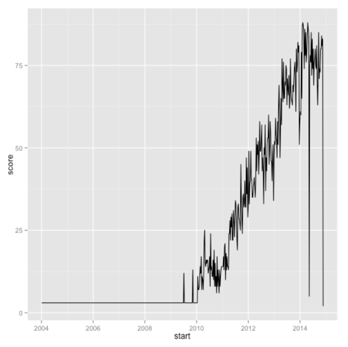
That’s much better but there is quite a bit of noise in the week to week scores which we can flatten a bit by plotting a rolling mean of the last 4 weeks instead:
> library(zoo)
> cleanGoogleTrends = cleanGoogleTrends %>%
    mutate(rolling = rollmean(score, 4, fill = NA, align=c("right")),
           start =  as.Date(start))

> ggplot(aes(x = start, y = rolling), data = cleanGoogleTrends) +
    geom_line(size = 0.5)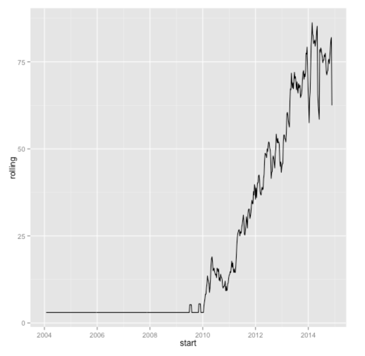
Here’s the full code if you want to reproduce:
library(dplyr)
library(zoo)
library(ggplot2)

googleTrends = read.csv("/Users/markneedham/Downloads/report.csv", row.names=NULL)
names(googleTrends) = c("week", "score")

cleanGoogleTrends = googleTrends %>%
  mutate(ind = row_number()) %>%
  group_by(ind) %>%
  mutate(dates = strsplit(week, " - "),
         start = dates[[1]][1] %>% strptime("%Y-%m-%d") %>% as.character(),
         end =   dates[[1]][2] %>% strptime("%Y-%m-%d") %>% as.character()) %>%
  filter(!is.na(start) | !is.na(end)) %>%
  ungroup() %>%
  select(-c(ind, dates, week)) %>%
  mutate(start =  as.Date(start),
         score = as.numeric(score),
         rolling = rollmean(score, 4, fill = NA, align=c("right")))

ggplot(aes(x = start, y = rolling), data = cleanGoogleTrends) +
  geom_line(size = 0.5)
My next step is to plot the Google Trends scores against my meetup data set to see if there’s any interesting correlations going on.
As an aside I made use of knitr while putting together this post – it works really well for checking that you’ve included all the steps and that it actually works!
| Reference: | R: Cleaning up and plotting Google Trends data from our JCG partner Mark Needham at the Mark Needham Blog blog. |
