Queueing Theory
The queueing theory allows us to predict queue lengths and waiting times, which is of paramount importance for capacity planning. For an architect this is a very handy tool, since queues are not just the appanage of messaging systems.
To avoid system over loading we use throttling. Whenever the number of incoming requests surpasses the available resources, we basically have two options:
- discarding all overflowing traffic, therefore decreasing availability
- queuing requests and wait (for as long as a time out threshold) for busy resources to become available
This behaviour applies to thread-per-request web servers, batch processors or connection pools.
What’s in it for us?
Agner Krarup Erlang is the father of queueing theory and traffic engineering, being the first to postulated the mathematical models required to provisioning telecommunication networks.
Erlang formulas are modelled for M/M/k queue models, meaning the system is characterized by:
- the arrival rate (λ) following a Poisson distribution
- the service times following an exponential distribution
- FIFO request queueing
The Erlang formulas give us the servicing probability for:
This is not strictly applicable to thread pools, as requests are not fairly serviced and servicing times not always follow an exponential distribution.
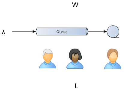
A general purpose formula, applicable to any stable system (a system where the arrival rate is not greater than the departure rate) is Little’s Law.

where
L – average number of customers
λ – long-term average arrival rate
W – average-time a request spends in a system
You can apply it almost everywhere, from shoppers queues to web request traffic analysis.
This can be regarded as a simple scalability formula, for to double the incoming traffic we have two options:
- reduce by half the response time (therefore increasing performance)
- double the available servers (therefore adding more capacity)
A real life example
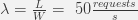
A simple example is a super-market waiting line. When you arrive at the line up you must pay attention to the arrival rate (e.g. λ = 2 persons / minute) and the queue length (e.g. L = 6 persons) to find out the amount of time you are going to spend waiting to be served (e.g. W = L / λ = 3 minutes).
A provisioning example
Let’s say we want to configure a connection pool to support a given traffic demand.
The connection pool system is characterized by the following variables:
Ws = service time (the connection acquire and hold time) = 100 ms = 0.1s
Ls = in-service requests (pool size) = 5
Assuming there is no queueing (Wq = 0):
Our connection pool can deliver up to 50 requests per second without ever queueing any incoming connection request.
Whenever there are traffic spikes we need to rely on a queue, and since we impose a fixed connection acquire timeout the queue length will be limited.
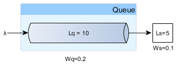
Since the system is considered stable the arrival rate applies both to the queue entry as for the actual services:
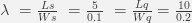
This queuing configuration still delivers 50 requests per second but it may queue 100 requests for 2 seconds as well, so a traffic burst of 150 requests lasting for 1 second would be manageable, since 50 requests can be served in the first second and the other 100 in following 2 seconds.
| Reference: | The simple scalability equation from our JCG partner Vlad Mihalcea at the Vlad Mihalcea’s Blog blog. |
