Time Series & Deep Learning (Part 2 of N): Data Preparation for Training and Evaluation of a LSTM
In the second post of this series we are going to learn how to prepare data for training and evaluation of a LSTM neural network for time series forecasting. Same as for any other post of this series I am referring to Python 3. The data set used is the same as for part 1.
LSTM (Long-Short Term Memory) neural networks are a specialization of RNNs (Recurrent Neural Networks) introduced by Sepp Hochreiter and Jurgen Schmiduber in 1997 to solve the problem of the Vanishing Gradient affecting RNNs. LSTMs are used in real-world applications of language translation, text generation, image captioning, music generation and time series forecasting. You can find more info about LSTMs in my book or wait for one of my next posts of this series. This post focuses mostly on one of the best practices for data preparation before using a data set for training and evaluation of a LSTM in a time series forecasting problem with the Keras library.
Let’s load the data set first:
from pandas import read_csv
from pandas import datetime

def parser(x):
    return datetime.strptime(x, '%Y-%m-%d')
features = ['date', 'value']
series = read_csv('./advance-retail-sales-building-materials-garden-equipment-and-supplies-dealers.csv', usecols=features, header=0, parse_dates=[1], index_col=1, squeeze=True, date_parser=parser)
The first action to do is to transform the time series in a way that the forecasting can be threat as a supervised learning problem. In supervised learning typically a data set is divided into input (containing the independent variables) and output (containing the target variable). We are going to use the observation from the previous time step (identified as t-1) as input and the observation at the current time step (identified as t) as output. No need to implement this transformation logic from scratch, as we can use the shift function available for pandas DataFrames. The input variables can be built by shifting of one place down all the values of the original time series. The output is the original time series. Finally we concatenate both series in a DataFrame. Because we need to apply this process to the values of the original data set, it would be good practice to implement a function for it:
from pandas import DataFrame
from pandas import concat

def tsToSupervised(series, lag=1):
    seriesDf = DataFrame(series)
    columns = [seriesDf.shift(idx) for idx in range(1, lag+1)]
    columns.append(seriesDf)
    seriesDf = concat(columns, axis=1)
    seriesDf.fillna(0, inplace=True)
    return seriesDf

supervisedDf = tsToSupervised(series, 1)
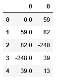
Here is a sample of how the supervised DataFrame looks like:
supervisedDf.head()
Is the data set now ready to be used to train and validate the network? Not yet. Other transformations need to be done. But this would be the topic of the next post.
The complete example would be released as a Jupyter notebook at the end of the first part of this series.
Published on Java Code Geeks with permission by Guglielmo Iozzia, partner at our JCG program. See the original article here: Time Series & Deep Learning (Part 2 of N): Data Preparation for Training and Evaluation of a LSTM Opinions expressed by Java Code Geeks contributors are their own. |
