Gianluca Bordello is an engineering manager at Sysdig, where he wears many hats. He’s a core developer of sysdig, an open source troubleshooting tool for Linux and containers, and spends his days dealing with backend development, performance analysis and cloud infrastructure management.
Introduction
As far as databases go, I’m a huge fan of Cassandra: it’s an incredibly powerful and flexible database that can ingest a massive amount of data while scaling across an arbitrary number of nodes. For these reasons, my team uses it very often for our internal applications.
But as with any piece of software, Cassandra has its own quirks and habits that you need to understand in order to effectively develop with it. In this article, I’ll show you a Cassandra performance issue that we recently dealt with, and I want to cover how we spotted the problem, what kind of troubleshooting we did to better understand it, and how we eventually solved it.
The Problem
One of our internal applications requires storing, and later processing, several thousands streams, where each stream consists of about a dozen binary blobs arriving periodically. Since we have many streams, and each blob can be fairly big (in the range of 10KB), we decided to use Cassandra 2.1 (a very stable version at the time of writing) and this very simple table:
CREATE TABLE streams (
	stream_id int,
	timestamp int,
	column0 blob,
	column1 blob,
	column2 blob,
	...
	column10 blob,
	primary key (stream_id, timestamp));
In this data model, all the blobs (10 in the above example) for a specific timestamp are stored in the same row, as separate columns. This allowed us to write a very simple application code, consisting essentially of a single write per stream during every period. Our typical read use case requires only one or two blobs at any given time. With this data model we have the flexibility of querying an arbitrary portion of the data with a single query, like this:
SELECT columnX from streams where stream_id=STREAM
For a while this schema worked well for us, and the response time we experienced for the database has been very good.
Recently we noticed deteriorated performance when querying streams containing particularly large blobs. Intuitively this would seem very reasonable since the data to be processed is larger, but there was something else that felt strange: despite the blobs being bigger in average, the specific ones we were retrieving in our queries were always roughly the same size as before.
In other words, it seemed as if Cassandra was always processing all 10 columns (including the large ones) despite us just asking for a particular, small column, thus causing degraded response times. This hypothesis seemed hard to believe at first, because Cassandra stores every single column separately, and there’s heavy indexing that allows you to efficiently lookup specific columns.
To validate our hypothesis, we wrote a separate test: in a table of N columns like ours, asking one single column should always take almost the same time regardless of the number and size of the other columns. With a little script (https://github.com/gianlucaborello/cassandra-benchmarks/blob/master/cassandra_benchmark_1.py), we got these results:
$ python ./cassandra_benchmark_1.py
Response time for querying a single column on a large table (column size 100 KB):
10 columns: 185 ms
20 columns: 400 ms
30 columns: 613 ms
40 columns: 668 ms
50 columns: 800 ms
60 columns: 1013 ms
70 columns: 1205 ms
80 columns: 1376 ms
90 columns: 1604 ms
100 columns: 1681 ms
We couldn’t have been more wrong! The tests proved the exact opposite of our assumption, and in fact the response time seemed to take a time directly proportional to the number of columns in the table, even if the query asked for just one of them!
Digging into Cassandra
In order to understand the problem better, I used sysdig, an open source troubleshooting tool. If you’re not familiar with sysdig, it has the ability to capture system state and activity from a running Linux instance, and then save, filter and analyze it. Think of sysdig as strace + tcpdump + htop + iftop + lsof in one.
Back to our story: I took a sysdig trace file while executing the same query of the previous test on a table with 100 columns:
SELECT column7 from streams where stream_id=1
This query returns a very small amount of data compared to the whole data set (around 10 MB), as sysdig can easily tell me by looking at the network activity generated by the database:
$ sysdig -r trace.scap -c topprocs_net
Bytes               Process             PID
--------------------------------------------------------------------------------
9.82M               java                34323
Despite this, the query takes almost 4 seconds to run, which is way more than what we want to wait in a similar scenario. Let’s take a look at the Cassandra file I/O activity while serving this single query:
$ sysdig -r trace.scap -c topfiles_bytes
Bytes               Filename
--------------------------------------------------------------------------------
971.04M
/var/lib/cassandra/data/benchmarks/test-23182450d5c011e5acecb7882d261790/benchmarks-te
st-ka-130-Data.db
538.80KB
/var/lib/cassandra/data/benchmarks/test-23182450d5c011e5acecb7882d261790/benchmarks-te
st-ka-130-Index.db
…
Wow, Cassandra seems to have read almost 1 GB from the file storing the data for my table, pretty much the whole size of the table:
$ du -hs /var/lib/cassandra/data/benchmarks/test-23182450d5c011e5acecb7882d261790/*
...
972M
/var/lib/cassandra/data/benchmarks/test-23182450d5c011e5acecb7882d261790/benchmarks-te
st-ka-130-Data.db
…
Which means that Cassandra essentially read the entire file, and this probably explains why the response time depends on the total number of columns of the table.
To take a deeper look, I used the spectrogram within csysdig on the I/O events over the duration of the trace file, so that we can visualize Cassandra’s latency and frequency of I/O operations:
$ csysdig -d 100 -r trace.scap -v spectro_file
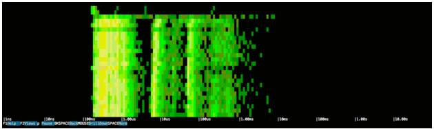
If you’re not familiar with a spectrogram, here’s the high level:
- It captures every system call (e.g. open, close, read, write, socket…) and it measures the call’s latency
- Every 100 ms it organizes the calls into buckets
- The spectrogram uses color to indicate how many calls are in each bucket
- Black means no calls during the last sample
- Shades of green mean 0 to 100 calls
- Shades of yellow mean hundreds of calls
- Shades of red mean thousands of calls or more
As a consequence, the left side of the diagram tends to show stuff that is fast, while the right side shows stuff that is slow.
What this image clearly tells us is that there seems to be a constant amount of I/O activity across the whole duration of the query, so, as predicted, accessing that 1 GB is likely what is negatively impacting the response time. Also, the latency of the I/O activity seems to be concentrated across two ranges, one very short (around 100 ns – 1 us) and one much more significant (around 10 us – 1 ms).
Let’s zoom into the band on the right, by selecting the area that I’m interested in exploring:
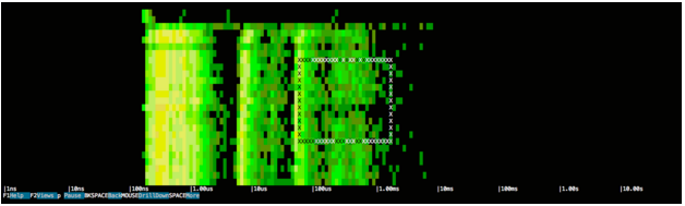
This selection will show the list of system events that match the time range and latency spectrum:

Read operations on the table file, tons of them. Indeed, this is essentially a full scan of the table done by reading it in chunks of 64 KB, and we can see how all those hundreds of microseconds blocked waiting for I/O add up in the final response time.
Solution: Cassandra Schema Refactor
We were pretty puzzled after discovering this behavior. As I mentioned before, rows and columns in Cassandra are heavily indexed, so we knew that there was no technical limitation for the query to not be served efficiently by reading exactly those 10 MB from disk instead of the full 1 GB.
Doing some research, we were able to find an issue (https://issues.apache.org/jira/browse/CASSANDRA-6586) describing this problem, and we understood that the behavior was meant to be that way in order to respect some semantics of the CQL query language adopted by Cassandra (omitted here for brevity, but clearly described in the issue), and the developers agreed this behavior could cause a significant performance penalty in cases like ours. While the issue is planned to be addressed in future versions of Cassandra, that left us with a bug in a production application that we had to somehow solve.
We opted for a workaround: since Cassandra will always read all the columns of a CQL row regardless of which ones are actually asked in a query, we decided to refactor our schema by shrinking the size of each row, and instead of putting all the blobs in the same row, we split them across multiple ones, like this:
CREATE TABLE streams (
	stream_id int,
	column_no int,
	timestamp int,
	column blob,
	primary key (stream_id, column_no, timestamp));
With this new schema all our rows are much smaller while still allowing us to efficiently query a single portion of the blob, with a query such as:
SELECT * from streams where stream_id=1 and column_no=7
This approach turned out to be quite effective: the query above that took 4 seconds with the old data model in the extreme test case, now took just around 100 ms on the same data set! It’s also interesting to analyze the new scenario with sysdig, and check Cassandra’s I/O while serving the request:
$ sysdig -r trace.scap -c topfiles_bytes
Bytes               Filename
--------------------------------------------------------------------------------
9.85M
/var/lib/cassandra/data/benchmarks/test-55d49260d5cb11e5acecb7882d261790/benchmarks-te
st-ka-16-Data.db
…
Just 10 MB, exactly the same size of the expected response. We can also use sysdig to answer the question: how did Cassandra know how to efficiently read the exact amount of data in a jungle of more than 1 GB? We can of course look at the system events done by the database process on the file:
$ sysdig -r trace.scap fd.filename=benchmarks-test-ka-16-Data.db
11285 15:13:40.896875243 1 java (34482) < open
fd=59(<f>/var/lib/cassandra/data/benchmarks/test-55d49260d5cb11e5acecb7882d261790/benc
hmarks-test-ka-16-Data.db)
name=/var/lib/cassandra/data/benchmarks/test-55d49260d5cb11e5acecb7882d261790/benchmarks-te
st-ka-16-Data.db flags=1(O_RDONLY) mode=0
11295 15:13:40.896926004 1 java (34482) > lseek
fd=59(<f>/var/lib/cassandra/data/benchmarks/test-55d49260d5cb11e5acecb7882d261790/benc
hmarks-test-ka-16-Data.db) offset=71986679 whence=0(SEEK_SET)
11296 15:13:40.896926200 1 java (34482) < lseek res=71986679
Here we see Cassandra opening the table file, but notice how immediately there’s a lseek operation that essentially skips in one single operation 70 MB of data, by setting the offset to the file descriptor with SEEK_SET to 71986679. This is essentially how typical “file indexing” works when observed from the system call point of view: Cassandra heavily relies on data structures to index the various contents of the table, so that it can move fast and efficiently to arbitrary and meaningful locations. In this case, the index contained the information that the columns with “stream_id=1” and “column_no=7” started at offset 71986679.
11400 15:13:40.898199496 1 java (34482) > read
fd=59(<f>/var/lib/cassandra/data/benchmarks/test-55d49260d5cb11e5acecb7882d261790/benc
hmarks-test-ka-16-Data.db) size=65798
11477 15:13:40.899058641 1 java (34482) < read res=65798
data=................................................................................
Right after jumping to the correct position of the file, we see normal sequential reads of 64 KB, in order to bring all the data into memory and process them. This loop of jumping to the right position and reading from it continues until all data (10 MB) is fully read.
It’s also quite interesting to see how this second case looks like in a spectrogram:
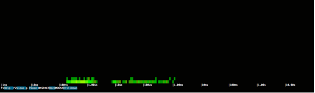
The spectrum of the I/O operations is pretty much the same as before and latencies are concentrated around the previous values, but notice how the height of the chart is completely different. This is because each horizontal line represents 100 ms of time, and since the whole query took about 100ms, the whole activity can be rendered in a much shorter chart. In other words, the height of the chart is directly proportional to the response time of Cassandra, so short means faster.
Conclusions
This story has two important messages into it, focused on monitoring and troubleshooting:
- Monitoring: Monitoring all the tiers of your infrastructure is very important. In this case, simply correlating the amount of data requested from Cassandra with the amount of I/O activity actually generated by the database helped us finding the cause of the problem, which we noticed in the first place by once again monitoring the response time of the queries.
- Troubleshooting: with sysdig, I’ve been able to dig into the specific behavior of Cassandra (e.g. confirming that the indexing was actually used by observing the lseek() activity) without even having to read its code and understand its internals, which for sure would have taken me more time. This concept is very powerful: if you already have some expectations of how a specific application is supposed to behave, observing its activity from the system call point of view can in many cases be an extremely effective way to do troubleshooting without spending a lot of time understanding less relevant details.
| Reference: | A tale of troubleshooting database performance, with Cassandra and sysdig from our JCG partner Gianluca Borello at the Planet Cassandra blog. |
