Graph Degree Distributions using R over Hadoop

Marko RodriguezJune 19th, 2014Last Updated: June 18th, 2014

0 38 6 minutes read

There are two common types of graph engines. One type is focused on providing real-time, traversal-based algorithms over linked-list graphs represented on a single-server. Such engines are typically called graph databases and some of the vendors include Neo4j, OrientDB, DEX, and InfiniteGraph. The other type of graph engine is focused on batch-processing using vertex-centric message passing within a graph represented across a cluster of machines. Graph engines of this form include Hama, Golden Orb, Giraph, and Pregel.

The purpose of this post is to demonstrate how to express the computation of two fundamental graph statistics — each as a graph traversal and as a MapReduce algorithm. The graph engines explored for this purpose are Neo4j and Hadoop. However, with respects to Hadoop, instead of focusing on a particular vertex-centric BSP-based graph-processing package such as Hama or Giraph, the results presented are via native Hadoop (HDFS + MapReduce). Moreover, instead of developing the MapReduce algorithms in Java, the R programming language is used. RHadoop is a small, open-source package developed by Revolution Analytics that binds R to Hadoop and allows for the representation of MapReduce algorithms using native R.

The two graph algorithms presented compute degree statistics: vertex in-degree and graph in-degree distribution. Both are related, and in fact, the results of the first can be used as the input to the second. That is, graph in-degree distribution is a function of vertex in-degree. Together, these two fundamental statistics serve as a foundation for more quantifying statistics developed in the domains of graph theory and network science.

Vertex in-degree: How many incoming edges does vertex X have?
Graph in-degree distribution: How many vertices have X number of incoming edges?

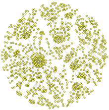
These two algorithms are calculated over an artificially generated graph that contains 100,000 vertices and 704,002 edges. A subset is diagrammed on the left. The algorithm used to generate the graph is called preferential attachment. Preferential attachment yields graphs with “natural statistics” that have degree distributions that are analogous to real-world graphs/networks. The respective iGraph R code is provided below. Once constructed and simplified (i.e. no more than one edge between any two vertices and no self-loops), the vertices and edges are counted. Next, the first five edges are iterated and displayed. The first edge reads, “vertex 2 is connected to vertex 0.” Finally, the graph is persisted to disk as a GraphML file.

~$ r

R version 2.13.1 (2011-07-08)
Copyright (C) 2011 The R Foundation for Statistical Computing

> g <- simplify(barabasi.game(100000, m=10))
> length(V(g))
[1] 100000
> length(E(g))
[1] 704002
> E(g)[1:5]
Edge sequence:
          
[1] 2 -> 0
[2] 2 -> 1
[3] 3 -> 0
[4] 4 -> 0
[5] 4 -> 1
> write.graph(g, '/tmp/barabasi.xml', format='graphml')

Graph Statistics using Neo4j

When a graph is on the order of 10 billion elements (vertices+edges), then a single-server graph database is sufficient for performing graph analytics. As a side note, when those analytics/algorithms are “ego-centric” (i.e. when the traversal emanates from a single vertex or small set of vertices), then they can typically be evaluated in real-time (e.g. < 1000 ms). To compute these in-degree statistics, Gremlin is used. Gremlin is a graph traversal language developed by TinkerPop that is distributed with Neo4j, OrientDB, DEX, InfiniteGraph, and the RDF engine Stardog. The Gremlin code below loads the GraphML file created by R in the previous section into Neo4j. It then performs a count of the vertices and edges in the graph.

~$ gremlin

         \,,,/
         (o o)
-----oOOo-(_)-oOOo-----
gremlin> g = new Neo4jGraph('/tmp/barabasi')
==>neo4jgraph[EmbeddedGraphDatabase [/tmp/barabasi]]
gremlin> g.loadGraphML('/tmp/barabasi.xml')
==>null
gremlin> g.V.count()
==>100000
gremlin> g.E.count()
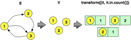
==>704002

The Gremlin code to calculate vertex in-degree is provided below. The first line iterates over all vertices and outputs the vertex and its in-degree. The second line provides a range filter in order to only display the first five vertices and their in-degree counts. Note that the clarifying diagrams demonstrate the transformations on a toy graph, not the 100,000 vertex graph used in the experiment.

gremlin> g.V.transform{[it, it.in.count()]}
...
gremlin> g.V.transform{[it, it.in.count()]}[0..4] 
==>[v[1], 99104]
==>[v[2], 26432]
==>[v[3], 20896]
==>[v[4], 5685]
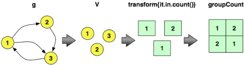
==>[v[5], 2194]

Next, to calculate the in-degree distribution of the graph, the following Gremlin traversal can be evaluated. This expression iterates through all the vertices in the graph, emits their in-degree, and then counts the number of times a particular in-degree is encountered. These counts are saved into an internal map maintained by groupCount. The final cap step yields the internal groupCount map. In order to only display the top five counts, a range filter is applied. The first line emitted says: “There are 52,611 vertices that do not have any incoming edges.” The second line says: “There are 16,758 vertices that have one incoming edge.”

gremlin> g.V.transform{it.in.count()}.groupCount.cap
...
gremlin> g.V.transform{it.in.count()}.groupCount.cap.next()[0..4]
==>0=52611
==>1=16758
==>2=8216
==>3=4805
==>4=3191

To calculate both statistics by using the results of the previous computation in the latter, the following traversal can be executed. This representation has a direct correlate to how vertex in-degree and graph in-degree distribution are calculated using MapReduce (demonstrated in the next section).

gremlin> degreeV = [:]
gremlin> degreeG = [:]
gremlin> g.V.transform{[it, it.in.count()]}.sideEffect{degreeV[it[0]] = it[1]}.transform{it[1]}.groupCount(degreeG)
...
gremlin> degreeV[0..4]
==>v[1]=99104
==>v[2]=26432
==>v[3]=20896
==>v[4]=5685
==>v[5]=2194
gremlin> degreeG.sort{a,b -> b.value <=> a.value}[0..4]
==>0=52611
==>1=16758
==>2=8216
==>3=4805
==>4=3191

Graph Statistics using Hadoop

When a graph is on the order of 100+ billion elements (vertices+edges), then a single-server graph database will not be able to represent nor process the graph. A multi-machine graph engine is required. While native Hadoop is not a graph engine, a graph can be represented in its distributed HDFS file system and processed using its distributed processing MapReduce framework. The graph generated previously is loaded up in R and a count of its vertices and edges is conducted. Next, the graph is represented as an edge list. An edge list (for a single-relational graph) is a list of pairs, where each pair is ordered and denotes the tail vertex id and the head vertex id of the edge. The edge list can be pushed to HDFS using RHadoop. The variable edge.list represents a pointer to this HDFS file.

> g <- read.graph('/tmp/barabasi.xml', format='graphml')
> length(V(g))
[1] 100000
> length(E(g))
[1] 704002
> edge.list <- to.dfs(get.edgelist(g))

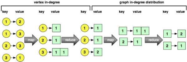
In order to calculate vertex in-degree, a MapReduce job is evaluated on edge.list. The map function is fed key/value pairs where the key is an edge id and the value is the ids of the tail and head vertices of the edge (represented as a list). For each key/value input, the head vertex (i.e. incoming vertex) is emitted along with the number 1. The reduce function is fed key/value pairs where the keys are vertices and the values are a list of 1s. The output of the reduce job is a vertex id and the length of the list of 1s (i.e. the number of times that vertex was seen as an incoming/head vertex of an edge). The results of this MapReduce job are saved to HDFS and degree.V is the pointer to that file. The final expression in the code chunk below reads the first key/value pair from degree.V — vertex 10030 has an in-degree of 5.

> degree.V <- mapreduce(edge.list, 
    map=function(k,v) keyval(v[2],1), 
    reduce=function(k,v) keyval(k,length(v)))
> from.dfs(degree.V)[[1]]
$key
[1] 10030
$val
[1] 5
attr(,"rmr.keyval")
[1] TRUE

In order to calculate graph in-degree distribution, a MapReduce job is evaluated on degree.V. The map function is fed the key/value results stored in degree.V. The function emits the degree of the vertex with the number 1 as its value. For example, if vertex 6 has an in-degree of 100, then the map function emits the key/value [100,1]. Next, the reduce function is fed keys that represent degrees with values that are the number of times that degree was seen as a list of 1s. The output of the reduce function is the key along with the length of the list of 1s (i.e. the number of times a degree of a particular count was encountered). The final code fragment below grabs the first key/value pair from degree.g — degree 1354 was encountered 1 time.

> degree.g <- mapreduce(degree.V, 
    map=function(k,v) keyval(v,1), 
    reduce=function(k,v) keyval(k,length(v)))
> from.dfs(degree.g)[[1]]
$key
[1] 1354
$val
[1] 1
attr(,"rmr.keyval")
[1] TRUE

In concert, these two computations can be composed into a single MapReduce expression.

> degree.g <- mapreduce(mapreduce(edge.list, 
    map=function(k,v) keyval(v[2],1), 
    reduce=function(k,v) keyval(k,length(v))), 
    map=function(k,v) keyval(v,1), 
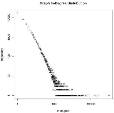
    reduce=function(k,v) keyval(k,length(v)))

Note that while a graph can be on the order of 100+ billion elements, the degree distribution is much smaller and can typically fit into memory. In general, edge.list > degree.V > degree.g. Due to this fact, it is possible to pull the degree.g file off of HDFS, place it into main memory, and plot the results stored within. The degree.g distribution is plotted on a log/log plot. As suspected, the preferential attachment algorithm generated a graph with natural “scale-free” statistics — most vertices have a small in-degree and very few have a large in-degree.

> degree.g.memory <- from.dfs(degree.g)
> plot(keys(degree.g.memory), values(degree.g.memory), log='xy', main='Graph In-Degree Distribution', xlab='in-degree', ylab='frequency')